The integration of information from heterogeneous web sources is of central interest for applications such as catalog data integration and warehousing of web data (e.g., job advertisements and announcements). Such data is typically textual and can be obtained from disparate web sources in a variety of ways, including web site crawling and direct access to remote databases via web protocols. The integration of such web data exhibits many semantics- and performance-related challenges.
Consider a price-comparison web site, backed by a database, that combines product information from different vendor web sites and presents the results under a uniform interface to the user. In such a situation, one cannot assume the existence of global identifiers (i.e., unique keys) for products across the autonomous vendor web sites. This raises a fundamental problem: different vendors may use different names to describe the same product. For example, a vendor might list a hard disk as ``Western Digital 120Gb 7200 rpm,'' while another might refer to the same disk as ``Western Digiral HDD 120Gb'' (due to a spelling mistake) or even as ``WD 120Gb 7200rpm'' (using an abbreviation). A simple equality comparison on product names will not properly identify these descriptions as referring to the same entity. This could result in the same product entity from different vendors being treated as separate products, defeating the purpose of the price-comparison web site. To effectively address the integration problem, one needs to match multiple textual descriptions, accounting for:
or combinations thereof.
Any attempt to address the integration problem has to specify a measure that effectively quantifies ``closeness'' or ``similarity'' between string attributes. Such a similarity metric can help establish that ``Microsoft Windows XP Professional'' and ``Windows XP Pro'' correspond to the same product across the web sites/databases, and that these are different from the ``Windows NT'' product. Many approaches to data integration use a text matching step, where similar textual entries are matched together as potential duplicates. Although text matching is an important component of such systems [1,21,23], little emphasis has been paid on the efficiency of this operation.
Once a text similarity metric is specified, there is a clear requirement for algorithms that process the data from the multiple sources to identify all pairs of strings (or sets of strings) that are sufficiently similar to each other. We refer to this operation as a text join. To perform such a text join on data originating at different web sites, we can utilize ``web services'' to fully download and materialize the data at a local relational database management system (RDBMS). Once this materialization has been performed, problems and inconsistencies can be handled locally via text join operations. It is desirable for scalability and effectiveness to fully utilize the RDBMS capabilities to execute such operations.
In this paper, we present techniques for performing text joins efficiently and robustly in an unmodified RDBMS. Our text joins rely on the cosine similarity metric [20], which has been successfully used in the past in the WHIRL system [4] for a similar data integration task. Our contributions include:
The remainder of this paper is organized as follows. Section 2 presents background and notation necessary for the rest of the discussion, and introduces a formal statement of our problem. Section 3 presents SQL statements to preprocess relational tables so that we can apply the sampling-based text join algorithm of Section 4. Then, Section 5 presents the implementation of the text join algorithm in SQL. A preliminary version of Sections 3 and 5 appears in [12]. Section 6 reports a detailed experimental evaluation of our techniques in terms of both accuracy and performance, and in comparison with other applicable approaches. Section 7 discusses the relative merits of alternative string similarity metrics. Section 8 reviews related work. Finally, Section 9 concludes the paper and discusses possible extensions of our work.
In this section, we first provide notation and background for text joins, which we follow with a formal definition of the problem on which we focus in this paper.
We denote with ![]() the
set of all strings over an alphabet
the
set of all strings over an alphabet ![]() . Each
string in
. Each
string in ![]() can be decomposed into a
collection of atomic ``entities'' that we generally refer to as
tokens. What constitutes a token can be defined in a
variety of ways. For example, the tokens of a string could
simply be defined as the ``words'' delimited by special
characters that are treated as ``separators'' (e.g., ` ').
Alternatively, the tokens of a string could correspond to all
of its
can be decomposed into a
collection of atomic ``entities'' that we generally refer to as
tokens. What constitutes a token can be defined in a
variety of ways. For example, the tokens of a string could
simply be defined as the ``words'' delimited by special
characters that are treated as ``separators'' (e.g., ` ').
Alternatively, the tokens of a string could correspond to all
of its ![]() -grams,
which are overlapping substrings of exactly
-grams,
which are overlapping substrings of exactly ![]() consecutive characters, for a given
consecutive characters, for a given ![]() . Our
forthcoming discussion treats the term token as generic, as the
particular choice of token is orthogonal to the design of our
algorithms. Later, in Section 6 we
experiment with different token definitions, while in
Section 7 we discuss the
effect of token choice on the characteristics of the resulting
similarity function.
. Our
forthcoming discussion treats the term token as generic, as the
particular choice of token is orthogonal to the design of our
algorithms. Later, in Section 6 we
experiment with different token definitions, while in
Section 7 we discuss the
effect of token choice on the characteristics of the resulting
similarity function.
Let ![]() and
and ![]() be two
relations with the same or different attributes and schemas. To
simplify our discussion and notation we assume, without loss of
generality, that we assess similarity between the entire sets
of attributes of
be two
relations with the same or different attributes and schemas. To
simplify our discussion and notation we assume, without loss of
generality, that we assess similarity between the entire sets
of attributes of ![]() and
and ![]() . Our
discussion extends to the case of arbitrary subsets of
attributes in a straightforward way. Given tuples
. Our
discussion extends to the case of arbitrary subsets of
attributes in a straightforward way. Given tuples ![]() and
and ![]() , we
assume that the values of their attributes are drawn from
, we
assume that the values of their attributes are drawn from ![]() . We adopt the widely used
vector-space retrieval model [20] from the
information retrieval field to define the textual similarity
between
. We adopt the widely used
vector-space retrieval model [20] from the
information retrieval field to define the textual similarity
between ![]() and
and ![]() .
.
Let ![]() be the (arbitrarily ordered) set of all unique
tokens present in all values of attributes of both
be the (arbitrarily ordered) set of all unique
tokens present in all values of attributes of both ![]() and
and
![]() .
According to the vector-space retrieval model, we conceptually
map each tuple
.
According to the vector-space retrieval model, we conceptually
map each tuple ![]() to a vector
to a vector
![]() . The value of the
. The value of the
![]() -th
component
-th
component ![]() of
of ![]() is a real
number that corresponds to the weight of the
is a real
number that corresponds to the weight of the ![]() -th
token of
-th
token of ![]() in
in ![]() . Drawing an
analogy with information retrieval terminology,
. Drawing an
analogy with information retrieval terminology, ![]() is
the set of all terms and
is
the set of all terms and ![]() is a
document weight vector.
is a
document weight vector.
Rather than developing new ways to define the weight vector
![]() for a tuple
for a tuple ![]() , we exploit an instance of the
well-established tf.idf weighting scheme from the
information retrieval field. (tf.idf stands for ``term
frequency, inverse document frequency.'') Our choice is further
supported by the fact that a variant of this general weighting
scheme has been successfully used for our task by Cohen's WHIRL
system [4].
Given a collection of documents
, we exploit an instance of the
well-established tf.idf weighting scheme from the
information retrieval field. (tf.idf stands for ``term
frequency, inverse document frequency.'') Our choice is further
supported by the fact that a variant of this general weighting
scheme has been successfully used for our task by Cohen's WHIRL
system [4].
Given a collection of documents ![]() , a simple
version of the tf.idf weight for a term
, a simple
version of the tf.idf weight for a term ![]() and
a document
and
a document ![]() is defined as
is defined as
![]() , where
, where ![]() is the number of times that
is the number of times that
![]() appears in document
appears in document ![]() and
and ![]() is
is
![]() , where
, where ![]() is
the number of documents in the collection
is
the number of documents in the collection ![]() that
contain term
that
contain term ![]() . The tf.idf weight for a term
. The tf.idf weight for a term
![]() in a
document is high if
in a
document is high if ![]() appears a large
number of times in the document and
appears a large
number of times in the document and ![]() is a
sufficiently ``rare'' term in the collection (i.e., if
is a
sufficiently ``rare'' term in the collection (i.e., if ![]() 's
discriminatory power in the collection is potentially high).
For example, for a collection of company names, relatively
infrequent terms such as ``AT&T'' or ``IBM'' will have
higher idf weights than more frequent terms such as
``Inc.''
's
discriminatory power in the collection is potentially high).
For example, for a collection of company names, relatively
infrequent terms such as ``AT&T'' or ``IBM'' will have
higher idf weights than more frequent terms such as
``Inc.''
For our problem, the relation tuples are our ``documents,''
and the tokens in the textual attribute of the tuples are our
``terms.'' Consider the ![]() -th token
-th token ![]() in
in
![]() and
a tuple
and
a tuple ![]() from relation
from relation ![]() . Then
. Then ![]() is the number of times that
is the number of times that
![]() appears in
appears in ![]() . Also,
. Also, ![]() is
is
![]() , where
, where ![]() is
the total number of tuples in relation
is
the total number of tuples in relation ![]() that contain
token
that contain
token ![]() . The tf.idf weight for token
. The tf.idf weight for token ![]() in
tuple
in
tuple ![]() is
is
![]() . To simplify
the computation of vector similarities, we normalize vector
. To simplify
the computation of vector similarities, we normalize vector
![]() to
unit length in the Euclidean space after we define it. The
resulting weights correspond to the impact of the terms, as defined
in [24]. Note
that the weight vectors will tend to be extremely sparse for
certain choices of tokens; we shall seek to utilize this
sparseness in our proposed techniques.
to
unit length in the Euclidean space after we define it. The
resulting weights correspond to the impact of the terms, as defined
in [24]. Note
that the weight vectors will tend to be extremely sparse for
certain choices of tokens; we shall seek to utilize this
sparseness in our proposed techniques.
Since vectors are normalized, this measure corresponds to
the cosine of the angle between vectors ![]() and
and ![]() , and has values between 0 and 1. The
intuition behind this scheme is that the magnitude of a
component of a vector expresses the relative ``importance'' of
the corresponding token in the tuple represented by the vector.
Intuitively, two vectors are similar if they share many
important tokens. For example, the string ``ACME'' will be
highly similar to ``ACME Inc,'' since the two strings differ
only on the token ``Inc,'' which appears in many different
tuples, and hence has low weight. On the other hand, the
strings ``IBM Research'' and ``AT&T Research'' will have
lower similarity as they share only one relatively common
term.
, and has values between 0 and 1. The
intuition behind this scheme is that the magnitude of a
component of a vector expresses the relative ``importance'' of
the corresponding token in the tuple represented by the vector.
Intuitively, two vectors are similar if they share many
important tokens. For example, the string ``ACME'' will be
highly similar to ``ACME Inc,'' since the two strings differ
only on the token ``Inc,'' which appears in many different
tuples, and hence has low weight. On the other hand, the
strings ``IBM Research'' and ``AT&T Research'' will have
lower similarity as they share only one relatively common
term.
The following join between relations ![]() and
and ![]() brings together the tuples from these relations that are
``sufficiently close'' to each other, according to a
user-specified similarity threshold
brings together the tuples from these relations that are
``sufficiently close'' to each other, according to a
user-specified similarity threshold ![]() :
:
The text join ``correlates'' two relations for a given
similarity threshold ![]() . It can be
easily modified to correlate arbitrary subsets of attributes of
the relations. In this paper, we address the problem of
computing the text join of two relations efficiently and within an unmodified RDBMS:
. It can be
easily modified to correlate arbitrary subsets of attributes of
the relations. In this paper, we address the problem of
computing the text join of two relations efficiently and within an unmodified RDBMS:
In the sequel, we first describe our methodology for
deriving, in a preprocessing step, the vectors corresponding to
each tuple of relations ![]() and
and ![]() using relational operations and representations. We then
present a sampling-based solution for efficiently computing the
text join of the two relations using standard SQL in an
RDBMS.
using relational operations and representations. We then
present a sampling-based solution for efficiently computing the
text join of the two relations using standard SQL in an
RDBMS.
In this section, we describe how we define auxiliary relations to represent tuple weight vectors, which we later use in our purely-SQL text join approximation strategy.
As in Section 2, assume that we
want to compute the text join
![]() of two
relations
of two
relations ![]() and
and ![]() .
. ![]() is
the ordered set of all the tokens that appear in
is
the ordered set of all the tokens that appear in ![]() and
and
![]() . We
use SQL expressions to create the weight vector associated with
each tuple in the two relations. Since -for some choice of
tokens- each tuple is expected to contain only a few of the
tokens in
. We
use SQL expressions to create the weight vector associated with
each tuple in the two relations. Since -for some choice of
tokens- each tuple is expected to contain only a few of the
tokens in ![]() , the associated weight vector is sparse. We
exploit this sparseness and represent the weight vectors by
storing only the tokens with non-zero weight. Specifically, for
a choice of tokens (e.g., words or
, the associated weight vector is sparse. We
exploit this sparseness and represent the weight vectors by
storing only the tokens with non-zero weight. Specifically, for
a choice of tokens (e.g., words or ![]() -grams), we
create the following relations for a relation
-grams), we
create the following relations for a relation ![]() :
:
Given two relations ![]() and
and ![]() , we
can use the SQL statements in Figure 1 to generate relations R1Weights
and R2Weights with a compact representation of the
weight vector for the
, we
can use the SQL statements in Figure 1 to generate relations R1Weights
and R2Weights with a compact representation of the
weight vector for the ![]() and
and ![]() tuples. Only the non-zero tf.idf weights are stored in
these tables. Interestingly, RiWeights and
RiSum are the only tables that need to be preserved
for the computation of
tuples. Only the non-zero tf.idf weights are stored in
these tables. Interestingly, RiWeights and
RiSum are the only tables that need to be preserved
for the computation of
![]() that we
describe in the remainder of the paper: all other tables are
just necessary to construct RiWeights and
RiSum. The space overhead introduced by these tables
is moderate. Since the size of RiSum is bounded by the size of RiWeights, we just analyze the space
requirements for RiWeights.
that we
describe in the remainder of the paper: all other tables are
just necessary to construct RiWeights and
RiSum. The space overhead introduced by these tables
is moderate. Since the size of RiSum is bounded by the size of RiWeights, we just analyze the space
requirements for RiWeights.
Consider the case where ![]() -grams are the
tokens of choice. (As we will see, a good value is
-grams are the
tokens of choice. (As we will see, a good value is ![]() .)
Then each tuple
.)
Then each tuple ![]() of relation
of relation ![]() can contribute
up to approximately
can contribute
up to approximately ![]()
![]() -grams to
relation RiWeights, where
-grams to
relation RiWeights, where ![]() is the number of
characters in
is the number of
characters in ![]() . Furthermore, each tuple in RiWeights consists of a tuple id tid, the actual token (i.e.,
. Furthermore, each tuple in RiWeights consists of a tuple id tid, the actual token (i.e., ![]() -gram in this
case), and its associated weight.
Then, if
-gram in this
case), and its associated weight.
Then, if ![]() bytes are needed to represent tid and weight, the total size of relation RiWeights will not exceed
bytes are needed to represent tid and weight, the total size of relation RiWeights will not exceed
![]() , which is a (small) constant times the size of the original
table
, which is a (small) constant times the size of the original
table ![]() . If words are used as the token of
choice, then we have at most
. If words are used as the token of
choice, then we have at most
![]() tokens per tuple
in
tokens per tuple
in ![]() . Also, to store the token attribute of RiWeights we need no more than one byte
for each character in the
. Also, to store the token attribute of RiWeights we need no more than one byte
for each character in the ![]() tuples.
Therefore, we can bound the size of RiWeights by
tuples.
Therefore, we can bound the size of RiWeights by ![]() times the size of
times the size of ![]() . Again, in
this case the space overhead is linear in the size of the
original relation
. Again, in
this case the space overhead is linear in the size of the
original relation ![]() .
.
Given the relations R1Weights and
R2Weights, a baseline approach [13,18] to compute
![]() is shown in
Figure 2. This SQL statement
performs the text join by computing the similarity of each pair
of tuples and filtering out any pair with similarity less than
the similarity threshold
is shown in
Figure 2. This SQL statement
performs the text join by computing the similarity of each pair
of tuples and filtering out any pair with similarity less than
the similarity threshold ![]() . This
approach produces an exact answer to
. This
approach produces an exact answer to
![]() for
for ![]() . Unfortunately, as we will see in
Section 6, finding an exact answer
with this approach is prohibitively expensive, which motivates
the sampling-based technique that we describe next.
. Unfortunately, as we will see in
Section 6, finding an exact answer
with this approach is prohibitively expensive, which motivates
the sampling-based technique that we describe next.
The result of
![]() only contains
pairs of tuples from
only contains
pairs of tuples from ![]() and
and ![]() with similarity
with similarity ![]() or higher. Usually we are interested in
high values for threshold
or higher. Usually we are interested in
high values for threshold ![]() , which
should result in only a few tuples from
, which
should result in only a few tuples from ![]() typically
matching each tuple from
typically
matching each tuple from ![]() . The baseline
approach in Figure 2, however,
calculates the similarity of all pairs of tuples from
. The baseline
approach in Figure 2, however,
calculates the similarity of all pairs of tuples from ![]() and
and
![]() that share at least one token. As a result, this baseline
approach is inefficient: most of the candidate tuple pairs that
it considers do not make it to the final result of the text
join. In this section, we describe a sampling-based
technique [2]
to execute text joins efficiently, drastically reducing the
number of candidate tuple pairs that are considered during
query processing.
that share at least one token. As a result, this baseline
approach is inefficient: most of the candidate tuple pairs that
it considers do not make it to the final result of the text
join. In this section, we describe a sampling-based
technique [2]
to execute text joins efficiently, drastically reducing the
number of candidate tuple pairs that are considered during
query processing.
The sampling-based technique relies on the following
intuition:
![]() could be
computed efficiently if, for each tuple
could be
computed efficiently if, for each tuple ![]() of
of ![]() , we
managed to extract a sample from
, we
managed to extract a sample from ![]() containing
mostly tuples suspected to be highly similar to
containing
mostly tuples suspected to be highly similar to ![]() .
By ignoring the remaining (useless) tuples in
.
By ignoring the remaining (useless) tuples in ![]() , we
could approximate
, we
could approximate
![]() efficiently.
The key challenge then is how to define a sampling strategy
that leads to efficient text join executions while producing an
accurate approximation of the exact query results. The
discussion of the technique is organized as follows:
efficiently.
The key challenge then is how to define a sampling strategy
that leads to efficient text join executions while producing an
accurate approximation of the exact query results. The
discussion of the technique is organized as follows:
The sampling algorithm described in this section is an
instance of the approximate matrix multiplication algorithm
presented in [2], which computes an
approximation of the product
![]() , where each
, where each
![]() is
a numeric matrix. (In our problem,
is
a numeric matrix. (In our problem, ![]() .) The actual
matrix multiplication
.) The actual
matrix multiplication
![]() happens during
a preprocessing, off-line step. Then, the on-line part of the
algorithm works by processing the matrix
happens during
a preprocessing, off-line step. Then, the on-line part of the
algorithm works by processing the matrix ![]() row by row.
row by row.
Consider tuple ![]() with
its associated token weight vector
with
its associated token weight vector ![]() , and each
tuple
, and each
tuple ![]() with its associated token weight
vector
with its associated token weight
vector ![]() . When
. When ![]() is clear from
the context, to simplify the notation we use
is clear from
the context, to simplify the notation we use ![]() as shorthand for
as shorthand for
![]() . We extract a sample of
. We extract a sample of
![]() tuples of size
tuples of size ![]() for
for ![]() as
follows:
as
follows:
Let ![]() be the number of times that
be the number of times that ![]() appears in the sample of size
appears in the sample of size ![]() . It follows
that:
. It follows
that:
The proof of this theorem follows from an argument similar
to that in [2] and from the
observation that the mean of the process that generates ![]() is
is
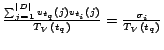 .
.
Theorem 1 establishes that, given
a tuple ![]() , we can obtain a sample of size
, we can obtain a sample of size
![]() of
tuples
of
tuples ![]() such that the frequency
such that the frequency ![]() of
tuple
of
tuple ![]() can be used to approximate
can be used to approximate ![]() . We can then report
. We can then report
![]() as part of the
answer of
as part of the
answer of
![]() for each
tuple
for each
tuple ![]() such that its estimated
similarity with
such that its estimated
similarity with ![]() (i.e., its estimated
(i.e., its estimated ![]() ) is
) is ![]() or larger,
where
or larger,
where
![]() is a threshold
slightly lower1
than
is a threshold
slightly lower1
than ![]() .
.
Given ![]() ,
, ![]() , and a
threshold
, and a
threshold ![]() , our discussion suggests the following
strategy for the evaluation of the
, our discussion suggests the following
strategy for the evaluation of the
![]() text join, in
which we process one tuple
text join, in
which we process one tuple ![]() at a
time:
at a
time:
This strategy guarantees that we can identify all pairs of
tuples with similarity of at least ![]() , with a
desired probability, as long as we choose an appropriate sample
size
, with a
desired probability, as long as we choose an appropriate sample
size ![]() . So far, the discussion has focused on
obtaining an
. So far, the discussion has focused on
obtaining an ![]() sample of size
sample of size ![]() individually
for each tuple
individually
for each tuple ![]() . A naive implementation of this
sampling strategy would then require a scan of relation
. A naive implementation of this
sampling strategy would then require a scan of relation ![]() for
each tuple in
for
each tuple in ![]() , which is clearly unacceptable in terms
of performance. In the next section we describe how the
sampling can be performed with only one sequential scan of
relation
, which is clearly unacceptable in terms
of performance. In the next section we describe how the
sampling can be performed with only one sequential scan of
relation ![]() .
.
As discussed so far, the sampling strategy requires
extracting a separate sample from ![]() for each tuple
in
for each tuple
in ![]() . This extraction of a potentially large
set of independent samples from
. This extraction of a potentially large
set of independent samples from ![]() (i.e., one per
(i.e., one per
![]() tuple) is of course inefficient, since it would require a large
number of scans of the
tuple) is of course inefficient, since it would require a large
number of scans of the ![]() table. In this
section, we describe how to adapt the original sampling
strategy so that it requires one single sample of
table. In this
section, we describe how to adapt the original sampling
strategy so that it requires one single sample of ![]() , following the
``presampling'' implementation in [2]. We then show how
to use this sample to create an approximate answer for the text
join
, following the
``presampling'' implementation in [2]. We then show how
to use this sample to create an approximate answer for the text
join
![]() .
.
As we have seen in the previous section, for each tuple
![]() we should sample a tuple
we should sample a tuple ![]() from
from ![]() in a way that depends on the
in a way that depends on the
![]() values. Since
these values are different for each tuple of
values. Since
these values are different for each tuple of ![]() , a
straightforward implementation of this sampling strategy
requires multiple samples of relation
, a
straightforward implementation of this sampling strategy
requires multiple samples of relation ![]() . Here we
describe an alternative sampling strategy that requires just
one sample of
. Here we
describe an alternative sampling strategy that requires just
one sample of ![]() : First, we sample
: First, we sample ![]() using only the
using only the ![]() weights from the tuples
weights from the tuples ![]() of
of ![]() , to
generate a single sample of
, to
generate a single sample of ![]() .
Then, we use the single sample differently for each tuple
.
Then, we use the single sample differently for each tuple ![]() of
of
![]() .
Intuitively, we ``weight'' the tuples in the sample according
to the weights
.
Intuitively, we ``weight'' the tuples in the sample according
to the weights ![]() of the
of the ![]() tuples of
tuples of
![]() . In
particular, for a desired sample size
. In
particular, for a desired sample size ![]() and a target
similarity
and a target
similarity ![]() , we realize the sampling-based text
join
, we realize the sampling-based text
join
![]() in three
steps:
in three
steps:
Such a sampling scheme identifies tuples with similarity
no less than ![]() from
from ![]() for each tuple
in
for each tuple
in ![]() . By sampling
. By sampling ![]() only once, the
sample will be correlated. As we verify experimentally in
Section 6, this sample correlation
has a negligible effect on the quality of the join
approximation.
only once, the
sample will be correlated. As we verify experimentally in
Section 6, this sample correlation
has a negligible effect on the quality of the join
approximation.
As presented, the join-approximation strategy is
asymmetric in the sense that it uses tuples from one
relation (![]() ) to weight samples obtained from the
other (
) to weight samples obtained from the
other (![]() ). The text join problem, as defined, is
symmetric and does not distinguish or impose an ordering on the
operands (relations). Hence, the execution of the text join
). The text join problem, as defined, is
symmetric and does not distinguish or impose an ordering on the
operands (relations). Hence, the execution of the text join
![]() naturally
faces the problem of choosing which relation to sample. For a
specific instance of the problem, we can break this asymmetry
by executing the approximate join twice. Thus, we first sample
from vectors of
naturally
faces the problem of choosing which relation to sample. For a
specific instance of the problem, we can break this asymmetry
by executing the approximate join twice. Thus, we first sample
from vectors of ![]() and use
and use ![]() to weight the
samples. Then, we sample from vectors of
to weight the
samples. Then, we sample from vectors of ![]() and
use
and
use ![]() to weight the samples. Then, we take the
union of these as our final result. We refer to this as a
symmetric text join. We will evaluate this technique
experimentally in Section 6.
to weight the samples. Then, we take the
union of these as our final result. We refer to this as a
symmetric text join. We will evaluate this technique
experimentally in Section 6.
In this section we have described how to approximate the
text join
![]() by using
weighted sampling. In the next section, we show how this
approximate join can be completely implemented in a standard,
unmodified RDBMS.
by using
weighted sampling. In the next section, we show how this
approximate join can be completely implemented in a standard,
unmodified RDBMS.
We now describe our SQL implementation of the sampling-based join algorithm of Section 4.2. Section 5.1 addresses the Sampling step, while Section 5.2 focuses on the Weighting and Thresholding steps for the asymmetric versions of the join. Finally, Section 5.3 discusses the implementation of a symmetric version of the approximate join.
Given the
![]() relations, we now show how
to implement the Sampling step of
the text join approximation strategy (Section 4.2) in SQL. For a desired sample
size
relations, we now show how
to implement the Sampling step of
the text join approximation strategy (Section 4.2) in SQL. For a desired sample
size ![]() and similarity threshold
and similarity threshold ![]() ,
we create the auxiliary relation shown in Figure 3. As the SQL statement in the figure
shows, we join the relations
,
we create the auxiliary relation shown in Figure 3. As the SQL statement in the figure
shows, we join the relations
![]() and
and
![]() on the token
attribute. The
on the token
attribute. The ![]() attribute for a tuple in the result is the
probability
attribute for a tuple in the result is the
probability
![]() with which we should pick this tuple (Section 4.2). Conceptually, for each tuple in
the output of the query of Figure 3 we need to perform
with which we should pick this tuple (Section 4.2). Conceptually, for each tuple in
the output of the query of Figure 3 we need to perform ![]() trials, picking each time the tuple with probability
trials, picking each time the tuple with probability ![]() .
For each successful trial, we insert the corresponding tuple
.
For each successful trial, we insert the corresponding tuple
![]() in a relation
in a relation
![]() , preserving
duplicates. The
, preserving
duplicates. The ![]() trials can be implemented in various ways.
One (expensive) way to do this is as follows: We add ``AND P
trials can be implemented in various ways.
One (expensive) way to do this is as follows: We add ``AND P
![]() RAND()'' in the WHERE clause of the Figure 3 query, so that the execution of this
query corresponds to one ``trial.'' Then, executing this query
RAND()'' in the WHERE clause of the Figure 3 query, so that the execution of this
query corresponds to one ``trial.'' Then, executing this query
![]() times and taking the union of the all results provides the
desired answer. A more efficient alternative, which is what we
implemented, is to open a cursor on the result of the query in
Figure 3, read one tuple at a
time, perform
times and taking the union of the all results provides the
desired answer. A more efficient alternative, which is what we
implemented, is to open a cursor on the result of the query in
Figure 3, read one tuple at a
time, perform ![]() trials on each tuple, and then write back
the result. Finally, a pure-SQL ``simulation'' of the Sampling step deterministically defines
that each tuple will result in Round(
trials on each tuple, and then write back
the result. Finally, a pure-SQL ``simulation'' of the Sampling step deterministically defines
that each tuple will result in Round(
![]() )
``successes'' after
)
``successes'' after ![]() trials, on
average. This deterministic version of the query is shown in
Figure 42. We have implemented and run
experiments using the deterministic version, and obtained
virtually the same performance as with the cursor-based
implementation of sampling over the Figure 3 query. In the rest of the paper -to
keep the discussion close to the probabilistic framework- we
use the cursor-based approach for the Sampling step.
trials, on
average. This deterministic version of the query is shown in
Figure 42. We have implemented and run
experiments using the deterministic version, and obtained
virtually the same performance as with the cursor-based
implementation of sampling over the Figure 3 query. In the rest of the paper -to
keep the discussion close to the probabilistic framework- we
use the cursor-based approach for the Sampling step.
|
|
|
|
Section 4.2 described the
Weighting and Thresholding steps as two separate steps.
In practice, we can combine them into one SQL statement, shown
in Figure 5. The Weighting step is implemented by the SUM
aggregate in the HAVING clause. We weight each tuple from the
sample according to
![]() ,
which corresponds to
,
which corresponds to
![]() (see
Section 4.2)3. Then, we can count the
number of times that each particular tuple pair appears in the
results (see GROUP BY clause). For each group, the result of
the SUM is the number of times
(see
Section 4.2)3. Then, we can count the
number of times that each particular tuple pair appears in the
results (see GROUP BY clause). For each group, the result of
the SUM is the number of times ![]() that a
specific tuple pair appears in the candidate set. To implement
the Thresholding step, we apply the
count filter as a simple comparison in the HAVING clause: we
check whether the frequency of a tuple pair at least matches the count
threshold (i.e.,
that a
specific tuple pair appears in the candidate set. To implement
the Thresholding step, we apply the
count filter as a simple comparison in the HAVING clause: we
check whether the frequency of a tuple pair at least matches the count
threshold (i.e.,
![]() ). The
final output of this SQL operation is a set of tuple id pairs
with expected similarity of at least
). The
final output of this SQL operation is a set of tuple id pairs
with expected similarity of at least ![]() .
The SQL statement in Figure 5 can be further simplified by
completely eliminating the join with the
.
The SQL statement in Figure 5 can be further simplified by
completely eliminating the join with the ![]() relation. The
relation. The ![]() values are used only in the HAVING
clause, to divide both parts of the inequality. The result of
the inequality is not affected by this division, hence the
values are used only in the HAVING
clause, to divide both parts of the inequality. The result of
the inequality is not affected by this division, hence the
![]() relation can be eliminated when combining the Weighting and the Thresholding step into one SQL
statement.
relation can be eliminated when combining the Weighting and the Thresholding step into one SQL
statement.
Up to now we have described only an asymmetric text join approximation
approach, in which we sample relation ![]() and weight the
samples according to the tuples in
and weight the
samples according to the tuples in ![]() (or vice
versa). However, as we described in Section 4.2, the text join
(or vice
versa). However, as we described in Section 4.2, the text join
![]() treats
treats ![]() and
and
![]() symmetrically. To break the asymmetry of our sampling-based
strategy, we execute the two different asymmetric
approximations and report the union of their results, as shown
in Figure 6. Note that a
tuple pair
symmetrically. To break the asymmetry of our sampling-based
strategy, we execute the two different asymmetric
approximations and report the union of their results, as shown
in Figure 6. Note that a
tuple pair
![]() that appears in
the result of the two intervening asymmetric approximations
needs high combined ``support'' to qualify in the final answer
(see HAVING clause in Figure 64).
that appears in
the result of the two intervening asymmetric approximations
needs high combined ``support'' to qualify in the final answer
(see HAVING clause in Figure 64).
An additional strategy naturally suggests itself: Instead of
executing the symmetric join algorithm by joining the samples
with the original relations, we can just join the samples, ignoring the original relations.
We sample each relation independently, join the samples, and
then weight and threshold the output. We implement the Weighting step by weighting each tuple
with
![]() . The count threshold in this case becomes
. The count threshold in this case becomes
![]() (again the
(again the ![]() values can be eliminated from the SQL
implementation if we combine the Weighting and the Thresholding steps). Figure 7 shows the SQL implementation of
this version of the sampling-based text join.
values can be eliminated from the SQL
implementation if we combine the Weighting and the Thresholding steps). Figure 7 shows the SQL implementation of
this version of the sampling-based text join.
We implemented the proposed SQL-based techniques and performed a thorough experimental evaluation in terms of both accuracy and performance in a commercial RDBMS. In Section 6.1, we describe the techniques that we compare and the data sets and metrics that we use for our experiments. Then, we report experimental results in Section 6.2.
We implemented the schema and the relations described in Section 3 in a commercial RDMBS, Microsoft SQL Server 2000, running on a multiprocessor machine with 2x2Ghz Xeon CPUs and with 2Gb of RAM. SQL Server was configured to potentially utilize the entire RAM as a buffer pool. We also compared our SQL solution against WHIRL, an alternative stand-alone technique, not available under Windows, using a PC with 2Gb of RAM, 2x1.8Ghz AMD Athlon CPUs and running Linux.
Data Sets: For our experiments, we used real
data from an AT&T customer relationship database. We
extracted from this database a random sample of 40,000 distinct attribute values of type string.
We then split this sample into two data sets, ![]() and
and
![]() .
Data set
.
Data set ![]() contains about 14,000 strings, while data
set
contains about 14,000 strings, while data
set ![]() contains about 26,000 strings. The
average string length for
contains about 26,000 strings. The
average string length for ![]() is 19
characters and, on average, each string consists of 2.5 words.
The average string length for
is 19
characters and, on average, each string consists of 2.5 words.
The average string length for ![]() is 21
characters and, on average, each string consists of 2.5 words.
The length of the strings follows a close-to-Gaussian
distribution for both data sets and is reported in
Figure 8(a), while the size of
is 21
characters and, on average, each string consists of 2.5 words.
The length of the strings follows a close-to-Gaussian
distribution for both data sets and is reported in
Figure 8(a), while the size of
![]() for different
similarity thresholds
for different
similarity thresholds ![]() and token
choices is reported in Figure 8(b).
We briefly discuss experiments over other data sets later in
this section.
and token
choices is reported in Figure 8(b).
We briefly discuss experiments over other data sets later in
this section.
|
Metrics: To evaluate the accuracy and completeness of our techniques we use the standard precision and recall metrics:
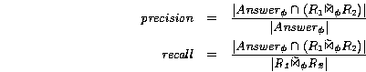
Precision and recall can take values in the 0-to-1 range.
Precision measures the accuracy of the answer and indicates the
fraction of tuples in the approximation of
![]() that are
correct. In contrast, recall measures the completeness of the
answer and indicates the fraction of the
that are
correct. In contrast, recall measures the completeness of the
answer and indicates the fraction of the
![]() tuples that
are captured in the approximation. We believe that recall is
more important than precision. The returned answer can always
be checked for false positives in a post-join step, while we
cannot locate false negatives without re-running the text join
algorithm.
tuples that
are captured in the approximation. We believe that recall is
more important than precision. The returned answer can always
be checked for false positives in a post-join step, while we
cannot locate false negatives without re-running the text join
algorithm.
Finally, to measure the efficiency of the algorithms, we measure the actual execution time of the text join for different techniques.
Choice of Tokens: We present experiments for different choices of tokens for the similarity computation. (Section 7 discusses the effect of the token choice on the resulting similarity function.) The token types that we consider in our experiments are:
The R1Weights table has 30,933
rows for Words, 268,458 rows for
Q-grams with ![]() ,
and 245,739 rows for Q-grams with
,
and 245,739 rows for Q-grams with
![]() .
For the R2Weights table, the
corresponding numbers of rows are 61,715, 536,982, and 491,515.
In Figure 8(b) we show the number
of tuple pairs in the exact result of the text join
.
For the R2Weights table, the
corresponding numbers of rows are 61,715, 536,982, and 491,515.
In Figure 8(b) we show the number
of tuple pairs in the exact result of the text join
![]() , for the
different token choices and for different similarity thresholds
, for the
different token choices and for different similarity thresholds
![]() .
.
Techniques Compared: We compare the following
algorithms for computing (an approximation of)
![]() . All of these
algorithms can be deployed completely within an RDBMS:
. All of these
algorithms can be deployed completely within an RDBMS:
In addition, we also compare the SQL-based techniques
against the stand-alone WHIRL system [4]. Given a
similarity threshold ![]() and two
relations
and two
relations ![]() and
and ![]() , WHIRL
computes the text join
, WHIRL
computes the text join
![]() . The
fundamental difference with our techniques is that WHIRL is a
separate application, not connected to any RDBMS. Initially, we
attempted to run WHIRL over our data sets using its default
settings. Unfortunately, during the computation of the
. The
fundamental difference with our techniques is that WHIRL is a
separate application, not connected to any RDBMS. Initially, we
attempted to run WHIRL over our data sets using its default
settings. Unfortunately, during the computation of the
![]() join WHIRL
ran out of memory. We then followed advice from WHIRL's
author [5] and
limited the maximum heap size 5 to produce an approximate answer for
join WHIRL
ran out of memory. We then followed advice from WHIRL's
author [5] and
limited the maximum heap size 5 to produce an approximate answer for
![]() . We measure
the precision and recall of the WHIRL answers, in addition to
the running time to produce them.
. We measure
the precision and recall of the WHIRL answers, in addition to
the running time to produce them.
WHIRL natively supports only word tokenization, but not
![]() -grams. To test WHIRL with
-grams. To test WHIRL with ![]() -grams, we adopted the following strategy:
We generated all the
-grams, we adopted the following strategy:
We generated all the ![]() -grams of the
strings in
-grams of the
strings in ![]() and
and ![]() , and stored
them as separate ``words.'' For example, the string ``ABC'' was
transformed into ``$A AB BC C#'' for
, and stored
them as separate ``words.'' For example, the string ``ABC'' was
transformed into ``$A AB BC C#'' for ![]() . Then WHIRL
used the transformed data set as if each
. Then WHIRL
used the transformed data set as if each ![]() -gram
were a separate word.
-gram
were a separate word.
Besides the specific choice of tokens, three other main
parameters affect the performance and accuracy of our
techniques: the sample size ![]() , the choice of
the user-defined similarity threshold
, the choice of
the user-defined similarity threshold ![]() , and the
choice of the error margin
, and the
choice of the error margin ![]() . We now
experimentally study how these parameters affect the accuracy
and efficiency of sampling-based text joins.
. We now
experimentally study how these parameters affect the accuracy
and efficiency of sampling-based text joins.
|
Comparing Different Techniques: Our first experiment
evaluates the precision and recall achieved by the different
versions of the sampling-based text joins and for WHIRL
(Figure 9). For sampling-based
joins, a sample size of ![]() is used (we
present experiments for varying sample size
is used (we
present experiments for varying sample size ![]() below). Figure 9(a) presents
the results for Words and
Figures 9(b)(c) present the
results for Q-grams, for
below). Figure 9(a) presents
the results for Words and
Figures 9(b)(c) present the
results for Q-grams, for ![]() and
and
![]() .
WHIRL has perfect precision (WHIRL computes the actual
similarity of the tuple pairs), but it demonstrates very low
recall for
.
WHIRL has perfect precision (WHIRL computes the actual
similarity of the tuple pairs), but it demonstrates very low
recall for ![]() -grams.
The low recall is, to some extent, a result of the small heap
size that we had to use to allow WHIRL to handle our data sets.
The sampling-based joins, on the other hand, perform better.
For Words, they achieve recall
higher than 0.8 for thresholds
-grams.
The low recall is, to some extent, a result of the small heap
size that we had to use to allow WHIRL to handle our data sets.
The sampling-based joins, on the other hand, perform better.
For Words, they achieve recall
higher than 0.8 for thresholds ![]() ,
with precision above 0.7 for most cases when
,
with precision above 0.7 for most cases when ![]() (with the exception of the
(with the exception of the ![]() technique). WHIRL has comparable
performance for
technique). WHIRL has comparable
performance for ![]() . For Q-grams with
. For Q-grams with ![]() ,
, ![]() has recall around 0.4 across different similarity thresholds,
with precision consistently above 0.7, outperforming WHIRL in
terms of recall across all similarity thresholds, except for
has recall around 0.4 across different similarity thresholds,
with precision consistently above 0.7, outperforming WHIRL in
terms of recall across all similarity thresholds, except for
![]() =0.9. When
=0.9. When ![]() ,
none of the algorithms performs well. For the sampling-based
text joins this is due to the small number of different tokens
for
,
none of the algorithms performs well. For the sampling-based
text joins this is due to the small number of different tokens
for ![]() . By comparing the different versions of
the sampling-based joins we can see that
. By comparing the different versions of
the sampling-based joins we can see that ![]() performs worse than the other
techniques in terms of precision and recall. Also,
performs worse than the other
techniques in terms of precision and recall. Also, ![]() is always worse than
is always worse than ![]() : Since
: Since
![]() is
larger than
is
larger than ![]() and the sample size is constant, the
sample of
and the sample size is constant, the
sample of ![]() represents the
represents the ![]() contents
better than the corresponding sample of
contents
better than the corresponding sample of ![]() does for
does for ![]() .
.
|
Effect of Sample Size ![]() : The second
set of experiments evaluates the effect of the sample size
(Figure 10). As we increase
the number of samples
: The second
set of experiments evaluates the effect of the sample size
(Figure 10). As we increase
the number of samples ![]() for each
distinct token of the relation, more tuples are sampled and
included in the final sample. This results in more matches in
the final join, and, hence in higher recall. It is also
interesting to observe the effect of the sample size for
different token choices. The recall for
for each
distinct token of the relation, more tuples are sampled and
included in the final sample. This results in more matches in
the final join, and, hence in higher recall. It is also
interesting to observe the effect of the sample size for
different token choices. The recall for ![]() -grams with
-grams with ![]() is smaller
than that for
is smaller
than that for ![]() -grams
with
-grams
with ![]() for a given sample size, which in turn is
smaller than the recall for Words.
Since we independently obtain a constant number of samples per
distinct token, the higher the number of distinct tokens the
more accurate the sampling is expected to be. This effect is
visible in the recall plots of Figure 10. The sample size also affects
precision. When we increase the sample size, precision
generally increases. However, in specific cases we can observe
that smaller sizes can in fact achieve higher precision. This
happens because for a smaller sample size we may get an underestimate of the similarity value
(e.g., estimated similarity 0.5 for real similarity 0.7).
Underestimates do not have a
negative effect on precision. However, an increase in the
sample size might result in an overestimate of the similarity, even if
the absolute estimation error is smaller (e.g., estimated
similarity 0.8 for real similarity 0.7). Overestimates, though,
affect precision negatively when the similarity threshold
for a given sample size, which in turn is
smaller than the recall for Words.
Since we independently obtain a constant number of samples per
distinct token, the higher the number of distinct tokens the
more accurate the sampling is expected to be. This effect is
visible in the recall plots of Figure 10. The sample size also affects
precision. When we increase the sample size, precision
generally increases. However, in specific cases we can observe
that smaller sizes can in fact achieve higher precision. This
happens because for a smaller sample size we may get an underestimate of the similarity value
(e.g., estimated similarity 0.5 for real similarity 0.7).
Underestimates do not have a
negative effect on precision. However, an increase in the
sample size might result in an overestimate of the similarity, even if
the absolute estimation error is smaller (e.g., estimated
similarity 0.8 for real similarity 0.7). Overestimates, though,
affect precision negatively when the similarity threshold ![]() happens to be between the real and the (over)estimated
similarity.
happens to be between the real and the (over)estimated
similarity.
Effect of Error Margin ![]() : As
mentioned in Section 4.1, the
threshold for count filter is
: As
mentioned in Section 4.1, the
threshold for count filter is
![]() . Different
values of
. Different
values of ![]() affect the precision and recall of
the answer. Figure 11 shows how
different choices of
affect the precision and recall of
the answer. Figure 11 shows how
different choices of ![]() affect
precision and recall. When we increase
affect
precision and recall. When we increase ![]() , we
lower the threshold for count filter and more tuple pairs are
included in the answer. This, of course, increases recall, at
the expense of precision: the tuple pairs included in the
result have estimated similarity
lower than the desired threshold
, we
lower the threshold for count filter and more tuple pairs are
included in the answer. This, of course, increases recall, at
the expense of precision: the tuple pairs included in the
result have estimated similarity
lower than the desired threshold ![]() . The choice
of
. The choice
of ![]() is an ``editorial'' decision, and
should be set to either favor recall or precision. As discussed
above, we believe that higher recall is more important: the
returned answer can always be checked for false positives in a
post-join step, while we cannot locate false negatives without
re-running the text join algorithm.
is an ``editorial'' decision, and
should be set to either favor recall or precision. As discussed
above, we believe that higher recall is more important: the
returned answer can always be checked for false positives in a
post-join step, while we cannot locate false negatives without
re-running the text join algorithm.
|
|
Execution Time: To analyze efficiency, we measure the
execution time of the different techniques. Our measurements do
not include the preprocessing step to build the auxiliary
tables in Figure 1: This
preprocessing step is common to the baseline and all
sampling-based text join approaches. This preprocessing step
took less than one minute to process both relations ![]() and
and
![]() for
Words, and about two minutes for
for
Words, and about two minutes for
![]() -grams.
Also, the time needed to create the RiSample relations is less than three
seconds. For WHIRL we similarly do not include the time needed
to export the relations from the RDBMS to a text file formatted
as expected by WHIRL, the time needed to load the text files
from disk, or the time needed to construct the inverted
indexes6.
The preprocessing time for WHIRL is about five seconds for
Words and thirty seconds for
-grams.
Also, the time needed to create the RiSample relations is less than three
seconds. For WHIRL we similarly do not include the time needed
to export the relations from the RDBMS to a text file formatted
as expected by WHIRL, the time needed to load the text files
from disk, or the time needed to construct the inverted
indexes6.
The preprocessing time for WHIRL is about five seconds for
Words and thirty seconds for ![]() -grams, which is smaller than for the
sampling-based techniques: WHIRL keeps the data in main memory,
while we keep the weights in materialized relations inside the
RDBMS.
-grams, which is smaller than for the
sampling-based techniques: WHIRL keeps the data in main memory,
while we keep the weights in materialized relations inside the
RDBMS.
The Baseline technique
(Figure 2) could only be run
for Words. For ![]() -grams, SQL Server executed the Baseline query for approximately 24
hours, using more than 60Gb of temporary disk space, without
producing any results. At that point we decided to stop the
execution. Hence, we only report results for Words for the Baseline technique.
-grams, SQL Server executed the Baseline query for approximately 24
hours, using more than 60Gb of temporary disk space, without
producing any results. At that point we decided to stop the
execution. Hence, we only report results for Words for the Baseline technique.
Figure 12(a) reports the
execution time of sampling-based text join variations for Words, for different sample sizes. The
execution time of the join did not change considerably for
different similarity thresholds 7, and is consistently lower
than that for Baseline. For
example, for ![]() , a sample size that results in high
precision and recall (Figure 10(a)),
, a sample size that results in high
precision and recall (Figure 10(a)), ![]() is more than
10 times faster than Baseline. The
speedup is even higher for
is more than
10 times faster than Baseline. The
speedup is even higher for ![]() and
and ![]() . Figures 12(b) and 12(c) report the execution time for
. Figures 12(b) and 12(c) report the execution time for ![]() -grams with
-grams with ![]() and
and ![]() .
Surprisingly,
.
Surprisingly, ![]() , which joins only the two samples, is
not faster than the other variations. For all choices of
tokens, the symmetric version
, which joins only the two samples, is
not faster than the other variations. For all choices of
tokens, the symmetric version ![]() has an
associated execution time that is longer than the sum of the
execution times of
has an
associated execution time that is longer than the sum of the
execution times of ![]() and
and ![]() . This is expected, since
. This is expected, since ![]() requires executing
requires executing ![]() and
and ![]() to compute its answer. Finally, Figure 12(d) reports the execution time for
WHIRL, for different similarity thresholds. (Note that WHIRL
was run on a slightly slower machine; see Section 6.1.) For
to compute its answer. Finally, Figure 12(d) reports the execution time for
WHIRL, for different similarity thresholds. (Note that WHIRL
was run on a slightly slower machine; see Section 6.1.) For ![]() -grams with
-grams with ![]() , the execution
time for WHIRL is roughly comparable to that of
, the execution
time for WHIRL is roughly comparable to that of ![]() when
when ![]() . For this setting
. For this setting ![]() has recall generally at or above 0.4, while WHIRL has recall
above 0.4 only for similarity threshold
has recall generally at or above 0.4, while WHIRL has recall
above 0.4 only for similarity threshold ![]() .
For Words, WHIRL is more efficient
than the sampling-based techniques for high values of
.
For Words, WHIRL is more efficient
than the sampling-based techniques for high values of ![]() ,
while WHIRL has significantly lower recall for low to moderate
similarity thresholds (Figure 9(a)). For example, for
,
while WHIRL has significantly lower recall for low to moderate
similarity thresholds (Figure 9(a)). For example, for ![]() sampling-based text joins have recall above 0.8 when
sampling-based text joins have recall above 0.8 when ![]() and WHIRL has recall above 0.8
only when
and WHIRL has recall above 0.8
only when ![]() .
.
Alternative Data Sets: We also
ran experiments for five additional data set pairs, ![]() through
through ![]() , using again real data from
different AT&T customer databases.
, using again real data from
different AT&T customer databases. ![]() consists of
two relations with approximately 26,000 and 260,000 strings
respectively. The respective numbers for the remaining pairs
are:
consists of
two relations with approximately 26,000 and 260,000 strings
respectively. The respective numbers for the remaining pairs
are: ![]() : 500 and 1,500 strings;
: 500 and 1,500 strings; ![]() :
26,000 and 1,500 strings;
:
26,000 and 1,500 strings; ![]() : 26,000 and
26,000 strings; and
: 26,000 and
26,000 strings; and ![]() : 30,000 and
30,000 strings.
: 30,000 and
30,000 strings.
Most of the results (reported in Figures 13 and 14) are analogous to those
for the data sets ![]() and
and ![]() .
The most striking difference is the extremely low recall for the
data set
.
The most striking difference is the extremely low recall for the
data set ![]() and similarity thresholds
and similarity thresholds ![]() and
and ![]() , for
, for
![]() -grams
with
-grams
with ![]() (Figure 13). This behavior is due to
peculiarities of the
(Figure 13). This behavior is due to
peculiarities of the ![]() data set:
data set:
![]() includes 7 variations of the string ``CompanyA
includes 7 variations of the string ``CompanyA ![]() ''8
(4 variations in each relation) that appear in a total of 2,160
and 204 tuples in each relation, respectively. Any pair of such
strings has real cosine similarity of at least 0.8. Hence the
text join contains many identical
tuple pairs with similarity of at least 0.8. Unfortunately, our
algorithm gives an estimated similarity of around 0.6 for 5 of
these pairs. This results in low recall for only 5 distinct tuple pairs that,
however, account for approximately 300,000 tuples in the join,
considerably hurting recall. Exactly the same problem appears
with 50 distinct entries of the form ``CompanyB
''8
(4 variations in each relation) that appear in a total of 2,160
and 204 tuples in each relation, respectively. Any pair of such
strings has real cosine similarity of at least 0.8. Hence the
text join contains many identical
tuple pairs with similarity of at least 0.8. Unfortunately, our
algorithm gives an estimated similarity of around 0.6 for 5 of
these pairs. This results in low recall for only 5 distinct tuple pairs that,
however, account for approximately 300,000 tuples in the join,
considerably hurting recall. Exactly the same problem appears
with 50 distinct entries of the form ``CompanyB ![]() '' (25 in each relation) that appear in
3,750 tuples in each relation. These tuples, when joined,
result in only 50 distinct tuple
pairs in the text join with similarity above 0.8 that again
account for 300,000 tuples in the join. Our algorithm
underestimates their similarity, which results in low recall
for similarity thresholds
'' (25 in each relation) that appear in
3,750 tuples in each relation. These tuples, when joined,
result in only 50 distinct tuple
pairs in the text join with similarity above 0.8 that again
account for 300,000 tuples in the join. Our algorithm
underestimates their similarity, which results in low recall
for similarity thresholds ![]() and
and
![]() .
.
|
|
In general, the sampling-based text joins, which are
executed in an unmodified RDBMS,
have efficiency comparable to WHIRL, when
WHIRL has sufficient main memory available: WHIRL is a
stand-alone application that implements a main-memory version
of the ![]() algorithm. This algorithm requires
keeping large search structures during processing; when main
memory is not sufficiently large for a data set, WHIRL's recall
suffers considerably. The
algorithm. This algorithm requires
keeping large search structures during processing; when main
memory is not sufficiently large for a data set, WHIRL's recall
suffers considerably. The ![]() strategy of
WHIRL could be parallelized [5], but a detailed
discussion of this is outside the scope of this paper. In
contrast, our techniques are fully executed within RDBMSs,
which are designed to handle large data volumes in
an efficient and scalable way.
strategy of
WHIRL could be parallelized [5], but a detailed
discussion of this is outside the scope of this paper. In
contrast, our techniques are fully executed within RDBMSs,
which are designed to handle large data volumes in
an efficient and scalable way.
Section 6 studied the accuracy and efficiency of text join executions, for different token choices and for a distance metric based on tf.idf token weights (Section 2). We now compare this distance metric against string edit distance, especially in terms of the effectiveness of the metrics in helping data integration applications.
The edit distance [16] between two strings is the minimum number of edit operations (i.e., insertions, deletions, and substitutions) of single characters needed to transform the first string into the second. The edit distance metric works very well for capturing typographical errors. For example, the strings ``Computer Science'' and ``Computer Scince'' have edit distance one. Also edit distance can capture insertions of short words (e.g., ``Microsoft'' and ``Microsoft Co'' have edit distance three). Unfortunately, a small increase of the distance threshold can capture many false matches, especially for short strings. For example, the string ``IBM'' is within edit distance three of both ``ACM'' and ``IBM Co.''
The simple edit distance metric does not work well when the compared strings involve block moves (e.g., ``Computer Science Department'' and ``Department of Computer Science''). In this case, we can use block edit distance, a more general edit distance metric that allows for block moves as a basic edit operation. By allowing for block moves, the block edit distance can also capture word rearrangements. Finding the exact block edit distance of two strings is an NP-hard problem [17]. Block edit distance cannot capture all mismatches. Differences between records also occur due to insertions and deletions of common words. For example, ``KAR Corporation International'' and ``KAR Corporation'' have block edit distance 14. If we allow large edit distance thresholds to capture such mismatches, the answer will contain a large number of false positive matches.
The insertion and deletion of common words can be handled effectively with the cosine similarity metric that we have described in this paper if we use words as tokens. Common words, like ``International,'' have low idf weight. Hence, two strings are deemed similar when they share many identical words (i.e., with no spelling mistakes) that do not appear frequently in the relation. This metric also handles block moves naturally. The use of words as tokens in conjunction with the cosine similarity as distance metric was proposed by WHIRL [4]. Unfortunately, this similarity metric does not capture word spelling errors, especially if they are pervasive and affect many of the words in the strings. For example, the strings ``Compter Science Department'' and ``Deprtment of Computer Scence'' will have zero similarity under this metric.
Hence, we can see that (block) edit distance and cosine similarity with words serve complementary purposes. Edit distance handles spelling errors well (and possibly block moves as well), while the cosine similarity with words nicely handles block moves and insertions of words.
A similarity function that naturally combines the good
properties of the two distance metrics is the cosine similarity
with ![]() -grams as tokens. A block move minimally
affects the set of common
-grams as tokens. A block move minimally
affects the set of common ![]() -grams of two
strings, so the two strings ``Gateway Communications'' and
``Communications Gateway'' have high similarity under this
metric. A related argument holds when there are spelling
mistakes in these words. Hence, ``Gteway Communications'' and
``Comunications Gateway'' will also have high similarity under
this metric despite the block move and the spelling errors in
both words. Finally, this metric handles the insertion and
deletion of words nicely. The string ``Gateway Communications''
matches with high similarity the string ``Communications
Gateway International'' since the
-grams of two
strings, so the two strings ``Gateway Communications'' and
``Communications Gateway'' have high similarity under this
metric. A related argument holds when there are spelling
mistakes in these words. Hence, ``Gteway Communications'' and
``Comunications Gateway'' will also have high similarity under
this metric despite the block move and the spelling errors in
both words. Finally, this metric handles the insertion and
deletion of words nicely. The string ``Gateway Communications''
matches with high similarity the string ``Communications
Gateway International'' since the ![]() -grams of the
word ``International'' appear often in the relation and have
low weight. Table 1
summarizes the qualitative properties of the distance functions
that we have described in this section.
-grams of the
word ``International'' appear often in the relation and have
low weight. Table 1
summarizes the qualitative properties of the distance functions
that we have described in this section.
The choice of similarity function impacts the execution time
of the associated text joins. The use of the cosine similarity
with words leads to fast query executions as we have seen in
Section 6. When we use ![]() -grams, the execution time of the join
increases considerably, resulting nevertheless in higher
quality of results with matches that neither edit distance nor
cosine similarity with words could have captured. Given the
improved recall and precision of the sampling-based text join
when
-grams, the execution time of the join
increases considerably, resulting nevertheless in higher
quality of results with matches that neither edit distance nor
cosine similarity with words could have captured. Given the
improved recall and precision of the sampling-based text join
when ![]() (compared to the case where
(compared to the case where ![]() ),
we believe that the cosine similarity metric with 3-grams can
serve well for data integration applications. A more thorough
study of the relative merits of the similarity metrics for
different applications is a subject of interesting future
work.
),
we believe that the cosine similarity metric with 3-grams can
serve well for data integration applications. A more thorough
study of the relative merits of the similarity metrics for
different applications is a subject of interesting future
work.
Integrating data from various sources is a problem that has attracted significant attention in different research communities. Various measures have been adopted to assess similarity or closeness between collections of entities to identify approximate matches.
In the statistical literature, the problem is referred to as the record linkage problem [8,25]. In this body of work similarity is quantified via a probabilistic framework that is aimed at minimizing the probability of ``misclassification,'' i.e., declaring two entities as different when they are actually the same. Learning the probabilities involves a training and a validation phase that can be quite complex to realize in practice. The bulk of work in this direction has concentrated on the modeling aspect, however, as opposed to on performance related issues. The typical assumption is that records fit in memory and/or that evaluation of the cross product of two files (and sometimes its materialization) is viable. This is not true with very large data collections.
Approximate matching of strings is a problem of central
interest for data integration and cleansing
applications [9,11]. The problem of
approximate string matching has attracted interest in the
algorithms and combinatorial pattern matching
communities [19] and commonly
the string edit distance (with its numerous variants)
is adopted for approximate string match quantification. Gravano
et al. [11]
presented a method to integrate approximate string match via
edit distance into a database and realize it as SQL statements.
They exploited a series of filters to speed join operations
between string attributes using the edit distance as a join
predicate. More specifically, this operation reports, for any
string in an attribute of a relation ![]() , all strings
in an attribute of a relation
, all strings
in an attribute of a relation ![]() that are
within a given edit distance. Hernández and
Stolfo [14] studied how
to identify approximate duplicate records in large databases.
Their approach relies on the ability to form a ``pseudo-key''
for each tuple by concatenating elements from its attributes.
Then, sorting and band joins [6] on the pseudo
keys can be used to identify approximate duplicates. Pseudo-key
formation is an application-dependent operation that requires
domain knowledge. Sarawagi and Bhamidipaty [21] describe an
active learning algorithm for combining different similarity
functions. The system is based on users to manually mark a
small set of ``potential duplicates'' as real duplicates or
not, and then uses these examples to optimize the combination
function. Cohen and Richman [3] use clustering in
conjunction with the cosine similarity metric to create
clusters of potential duplicate entries.
that are
within a given edit distance. Hernández and
Stolfo [14] studied how
to identify approximate duplicate records in large databases.
Their approach relies on the ability to form a ``pseudo-key''
for each tuple by concatenating elements from its attributes.
Then, sorting and band joins [6] on the pseudo
keys can be used to identify approximate duplicates. Pseudo-key
formation is an application-dependent operation that requires
domain knowledge. Sarawagi and Bhamidipaty [21] describe an
active learning algorithm for combining different similarity
functions. The system is based on users to manually mark a
small set of ``potential duplicates'' as real duplicates or
not, and then uses these examples to optimize the combination
function. Cohen and Richman [3] use clustering in
conjunction with the cosine similarity metric to create
clusters of potential duplicate entries.
The information retrieval field has produced approaches to speed up query execution that involve computation of the cosine similarity metric using inverted indexes [26]. A key idea is to exploit inverted indexes for fast computation of term weights. These techniques are of limited applicability for our approach: since we calculate and store the token weights during the preprocessing step of Section 3, we avoid the overhead of weight calculation during the join operation. However, we can apply some of these techniques to speedup the preprocessing step. Other optimizations described in [26] describe how to efficiently compute the document ``lengths'' to calculate the cosine similarity between documents. Since we use normalized weights, we do not have to calculate the document lengths on the fly. Additional optimizations, such as ``quantization of weights,'' [26] can be easily implemented inside a database system both for the baseline and for the sampling approach. Finally, some techniques also make special use of the available main memory to improve query-processing performance. These techniques are not compatible with our key objective of running the text joins in an unmodified RDBMS. Techniques that are based on the pruning of the inverted index [22,24] are close in spirit to our work, especially if we implement the sampling step using the ROUND function (Figure 4), which effectively prunes all the tokens with small weights.
Sampling has been utilized in a variety of tasks of database interest including data mining, estimation and optimization of queries, and query answering. A range of database vendors provide declarative interfaces that support a variety of sampling techniques inside the database engine [15]. Iceberg queries [7] utilize sampling for efficient answering of group-by queries. In particular, the techniques proposed by Fang et al. [7] utilize approximate counting techniques based on variants of hashing to efficiently estimate aggregate functions on groups of tuples.
Grossman et al. [13] present techniques for representing text documents and their associated term frequencies in relational tables, as well as for mapping boolean and vector-space queries into standard SQL queries. They also use a query-pruning technique, based on word frequencies, to speed up query execution. In this paper, we follow the same general approach of translating complex functionality not natively supported by a RDBMS into operations and queries that a RDBMS can optimize and execute efficiently. Grossman et al.'s technique can be adapted for our text join problem; we evaluate a version of this approach experimentally in Section 6.
Finally, the approximate matrix multiplication algorithm in [2] and Cohen's WHIRL system [4] are closest to our work, and have been discussed in Sections 4 and 6, respectively. In particular, Section 4 summarizes the strategy in [2] as applied to our problem.
In this paper, we studied the problem of matching textual attributes that refer to the same entity. For this, we adopted the well established measure of cosine similarity over the vector-space retrieval model and proposed a SQL implementation of a sampling-based strategy to compute text joins in an unmodified RDBMS. Our algorithms are approximate, and we experimentally evaluated the accuracy/performance tradeoffs.
The work presented herein raises various issues for further study. As a notable example, conducting a thorough qualitative study of the properties of the different similarity functions for data integration applications is an interesting piece of future work.
![\fbox{ \begin{tabular}{ll} \begin{minipage}[t]{3in} \begin{tabbing} {\tt INS... ...oken weights & (f) Dummy relation used to create \emph{RiIDF} \end{tabular} }](p627-gravanoimg57.png)
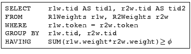
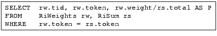
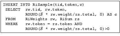
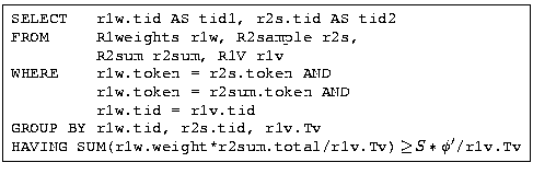
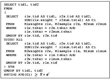
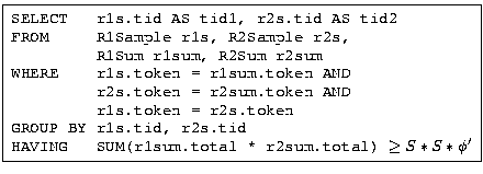
![\includegraphics[width=0.9\columnwidth]{figs/lengths.eps}](p627-gravanoimg128.png)
![\includegraphics[width=0.9\columnwidth]{figs/distances.eps}](p627-gravanoimg129.png)
![\includegraphics[width=0.33\textwidth]{figs/sym-asym-words-precision.eps}](p627-gravanoimg135.png)
![\includegraphics[width=0.33\textwidth]{figs/sym-asym-q2-precision.eps}](p627-gravanoimg136.png)
![\includegraphics[width=0.33\textwidth]{figs/sym-asym-q3-precision.eps}](p627-gravanoimg137.png)
![\includegraphics[width=0.33\textwidth]{figs/sym-asym-words-recall.eps}](p627-gravanoimg138.png)
![\includegraphics[width=0.33\textwidth]{figs/sym-asym-q2-recall.eps}](p627-gravanoimg139.png)
![\includegraphics[width=0.33\textwidth]{figs/sym-asym-q3-recall.eps}](p627-gravanoimg140.png)
![\includegraphics[width=0.33\textwidth]{figs/sam-words-precision.eps}](p627-gravanoimg144.png)
![\includegraphics[width=0.33\textwidth]{figs/sam-q2-precision.eps}](p627-gravanoimg145.png)
![\includegraphics[width=0.33\textwidth]{figs/sam-q3-precision.eps}](p627-gravanoimg146.png)
![\includegraphics[width=0.33\textwidth]{figs/sam-words-recall.eps}](p627-gravanoimg147.png)
![\includegraphics[width=0.33\textwidth]{figs/sam-q2-recall.eps}](p627-gravanoimg148.png)
![\includegraphics[width=0.33\textwidth]{figs/sam-q3-recall.eps}](p627-gravanoimg149.png)
![\includegraphics[width=0.7\columnwidth]{figs/epsilon-q3-precision.eps}](p627-gravanoimg151.png)
![\includegraphics[width=0.7\columnwidth]{figs/epsilon-q3-recall.eps}](p627-gravanoimg152.png)
![\includegraphics[width=0.36\textwidth]{figs/timing-words.eps}](p627-gravanoimg154.png)
![\includegraphics[width=0.36\textwidth]{figs/timing-q3.eps}](p627-gravanoimg155.png)
![\includegraphics[width=0.36\textwidth]{figs/timing-q2.eps}](p627-gravanoimg156.png)
![\includegraphics[width=0.36\textwidth]{figs/timing-whirl.eps}](p627-gravanoimg157.png)
![\includegraphics[width=0.7\columnwidth]{figs/alternativesets-precision.eps}](p627-gravanoimg167.png)
![\includegraphics[width=0.7\columnwidth]{figs/alternativesets-recall.eps}](p627-gravanoimg168.png)
![\includegraphics[width=0.7\columnwidth]{figs/alternativesets-precision-words.eps}](p627-gravanoimg169.png)
![\includegraphics[width=0.7\columnwidth]{figs/alternativesets-recall-words.eps}](p627-gravanoimg170.png)