|
|
A Combinatorial Allocation Mechanism With Penalties For Banner Advertising
Uriel Feige |
Nicole Immorlica |
Vahab S. Mirrokni |
Hamid Nazerzadeh |
|
|
ABSTRACT
Most current banner advertising is sold through negotiation thereby incurring large transaction costs and possibly suboptimal allocations. We propose a new automated system for selling banner advertising. In this system, each advertiser specifies a collection of host webpages which are relevant to his product, a desired total quantity of impressions on these pages, and a maximum per-impression price. The system selects a subset of advertisers as winners and maps each winner to a set of impressions on pages within his desired collection. The distinguishing feature of our system as opposed to current combinatorial allocation mechanisms is that, mimicking the current negotiation system, we guarantee that winners receive at least as many advertising opportunities as they requested or else receive ample compensation in the form of a monetary payment by the host. Such guarantees are essential in markets like banner advertising where a major goal of the advertising campaign is developing brand recognition.
As we show, the problem of selecting a feasible subset of advertisers with maximum total value is inapproximable. We thus present two greedy heuristics and discuss theoretical techniques to measure their performances. Our first algorithm iteratively selects advertisers and corresponding sets of impressions which contribute maximum marginal per-impression profit to the current solution. We prove a bi-criteria approximation for this algorithm, showing that it generates approximately as much value as the optimum algorithm on a slightly harder problem. However, this algorithm might perform poorly on instances in which the value of the optimum solution is quite large, a clearly undesirable failure mode. Hence, we present an adaptive greedy algorithm which again iteratively selects advertisers with maximum marginal per-impression profit, but additionally reassigns impressions at each iteration. For this algorithm, we prove a structural approximation result, a newly defined framework for evaluating heuristics []FIMN08. We thereby prove that this algorithm has a better performance guarantee than the simple greedy algorithm.
Categories and Subject Descriptors
F.2 [Theory of Computation]: Analysis of Algorithms and Problem Complexity; J.4 [Computer Applications]: Social and Behavioral Sciences—Economics
General Terms
Algorithm, Theory, Economics
Keywords
Internet Advertising, Supply Guarantee, Combinatorial Auctions, Structural Approximation
1. Online advertising is one of the most profitable business models for Internet services to date, accounting for annual revenues approaching $17 billion dollars according to the Internet Advertising Bureau [21]. According to the same report, 22% of this revenue comes from banner advertising, or graphic-based advertisements which appear embedded in content pages on a host website. Current models of banner advertising require advertisers to negotiate rates directly with the sales representatives of the host on a monthly basis. These negotiations involve several parameters. First, the advertiser specifies a subset of content pages which are relevant to his or her ad. Next, the advertiser requests a desired number of impressions, or advertising opportunities, on pages from among his or her specified subset, and a per-impression price. Finally, if the negotiation is successful and the contract is accepted, the advertisement is shown on some subset of the specified content pages. By accepting a contract the supplier is committed to the supply. If the supply is not met, the bidder is compensated in two ways: he is not charged for the parts that are not met, and moreover, he gets them for free in the next time period.
This process requires a lot of overhead for advertisers who must negotiate with sales representatives, and a lot of guess-work for sales representatives who must decide based on intuition which advertising contracts to accept. As a result, small advertisers tend to be locked out of the system, unable to bear the cost of the smallest-sized contracts, and the system overall suffers additional inefficiencies from the suboptimal decisions of the sales representatives. In this paper, we consider automating this system. We design a system which each month considers the supply of page views and a set of bids, each specifying a desired set of pages, a desired number of impressions, and a per-impression value, and then selects a subset of bids which maximizes the value while sustaining penalties for under-allocated impressions. Whereas in practice, the penalties are realized in the form of free impressions, in our system we represent these penalties with a monetary payment from the host to the advertiser equal to a specified multiple of the per-impression value for each under-allocated impression. The penalty factor reflects an estimate of how much next month's impressions are going to be worth.
There are several factors which make this system harder to design than general combinatorial allocation mechanisms. The most significant difference comes from the fact that the host must ``guarantee'' supply by paying a penalty for under-allocated impressions. Such guarantees are quite characteristic of the banner advertising market, and are important in branding campaigns where it is essential for the advertiser to receive at least some minimum number of impressions - the McDonald's arches or the Nike swoosh are recognizable precisely because they are ubiquitous. However, these guarantees also make the underlying optimization problem hard to approximate: for example, if the penalty is very large, then each winner must receive all of his requested impressions and so we can reduce our problem from the well-known set packing problem [15]. In fact, as we show, even for small penalties, our problem is not approximable within any constant factor.
We therefore focus on designing heuristics with varying sorts of
provable guarantees. A common approach to combat inapproximability is
to develop bi-criteria approximations, or algorithms that do
almost as well as the optimum solution on a slightly harder problem.
For example, in ![]() -balanced graph partitioning, the goal is to
cut the minimum number of edges to divide a graph on
-balanced graph partitioning, the goal is to
cut the minimum number of edges to divide a graph on ![]() vertices into
two parts, each with at most
vertices into
two parts, each with at most ![]() vertices. The seminal paper of
Leighton and Rao [18] provides a bi-criteria approximation
algorithm for
vertices. The seminal paper of
Leighton and Rao [18] provides a bi-criteria approximation
algorithm for ![]() -balanced graph partitioning which cuts at most a
factor of
-balanced graph partitioning which cuts at most a
factor of ![]() more edges than the optimum solution on the
harder problem of bisection, or
more edges than the optimum solution on the
harder problem of bisection, or ![]() -balanced graph partitioning.
This was improved to
-balanced graph partitioning.
This was improved to
![]() by Arora et al. [3].
The bi-criteria framework has also been applied to min sum
clustering [5] and selfish routing [22].
by Arora et al. [3].
The bi-criteria framework has also been applied to min sum
clustering [5] and selfish routing [22].
In our case, we apply the bi-criteria framework by designing an
algorithm that does approximately as well as the optimum algorithm
with larger penalties. Our algorithm is extremely simple and trivial to
implement: it selects at each iteration a new winner and a
corresponding set of impressions with maximum marginal per-impression
profit. We show that this algorithm gets at least 23% of the optimum
profit on a problem with ![]() times the penalty (i.e., whereas our
algorithm just pays an advertiser his per-impression bid for each
under-allocated impression, the optimum must pay
times the penalty (i.e., whereas our
algorithm just pays an advertiser his per-impression bid for each
under-allocated impression, the optimum must pay ![]() times the
per-impression bid).
times the
per-impression bid).
Despite the bi-criteria guarantee, we note that this greedy algorithm may perform poorly when the optimum solution has large value. These are exactly the instances in which we would like to perform well. Hence, we present a refined greedy algorithm which involves solving a flow computation and prove guarantees on its performance in the structural approximation [10] framework, a newly developed framework for evaluating the approximation factor of heuristic algorithms. This framework allows one to evaluate the approximation factor of an algorithm based on the structure of the optimal (or any) solution, and not only the value of the optimal solution. In particular, it provides a performance guarantee that improves as the performance of the optimum solution improves, and unlike the bi-criteria framework, it provides these guarantees with respect to the optimum on the same problem instance.
Our refined greedy algorithm iteratively selects advertisers with maximum marginal per-impression profit, as before, but additionally considers re-allocating impressions to already selected advertisers at each step. In evaluating this algorithm, we consider the fraction of demand that the optimum satisfies for each advertiser. We show as this fraction increases, hence increasing the optimum value, our algorithm's value also increases. For example, if the optimum always satisfies 75% of the demand of each advertiser, then our algorithm gets at least 10% of the optimum, wherease if the optimum satsifies 99% of the demand of each advertiser, then our algorithm gets at least 30% of the value of the optimum. See Section 5.1 for the exact trade-off curve.
We note that the refined greedy algorithm outperforms the simple greedy algorithm on many classes of instances. However, this improved performance comes at the expense of increased difficulty in the implementation (and an additional linear factor in the running time).
In order to model the banner advertising problems and its key feature of supply guarantees, we make several enabling assumptions. First, we assume that the supply (i.e., monthly set of page views) is known and periodic. While in reality this supply is actually unknown, it is reasonable to assume that the host has good estimates of this supply and that the supply is fairly constant over time. Furthermore, the periodic supply assumption is essential if we intend to guarantee supply to advertisers. Second, while the real goal of the host is to optimize value over time, we instead focus on optimizing on a month-by-month basis. In other words, our stated goal is to maximize value this month with no regard to the effects on following months' revenues. Hence, for example, we assume that under-allocated supply for an advertiser (which will be offered for free the following month) costs our algorithm an amount equal to the advertiser's bid. This approach works well in situations in which the monthly demand is fairly static, a reasonable assumption in banner advertising scenarios. Third, and finally,
It is important to note that we ignore incentives throughout this work, i.e., we analyze the value of our allocation mechanism in an idealized world where advertisers truthfully report their types and not in an economic equilibrium. While incentive issues are very important in practice, they tend to have less effect in highly competitive settings. In successful banner advertising systems, where lots of advertisers compete for limited supply, we intuitively expect incentives to play a minimal role. We leave it as further work to study incentives in our proposed systems and/or calculate payments to make our proposed systems truthful.
In the context of Internet advertising, sponsored search auctions have
been studied extensively. The closest works to ours in this
literature are the ![]() -competitive algorithms that have
been designed for maximizing revenue for online allocation of
advertisement space [20,6,19].
-competitive algorithms that have
been designed for maximizing revenue for online allocation of
advertisement space [20,6,19].
Our work is distinguished from previous work in the literature by the existence of supply guarantees, implemented through penalties. These penalties reflect the non-linearity of bidder valuations, a characteristic of advertisers in banner advertising markets.
This paper is organized as follows. We give a formal definition of the model in Section 2. In this section, we also give the following basic observation about our problem: in the guaranteed banner advertisement problem, if the set of served advertisers is fixed, the optimal allocation can be found in polynomial time. This indicates that the challenging part of the problem is to find the set of advertisers that should be served to maximize the value. In Section 3, we prove that the problem does not admit a constant-factor approximation algorithm even for weak supply guarantee conditions. Next, in Section 4, we give a bi-criteria approximation algorithm for the problem. In Section 5, we give an adaptive greedy algorithm and analyze it in the structural approximation framework.
The banner advertisement problem can be modeled as follows.
We are given a set  of m advertisers {1,…,m} and a
set
of m advertisers {1,…,m} and a
set  of advertising opportunities that can be allocated
to them. Each advertising opportunity is an impression
of an advertisement on a webpage. For the rest of the
paper, we refer to each advertising opportunity as an item.
Without loss of generality, we assume all items of are
distinct. The bid of an advertiser i is a tuple (Ii,di,bi) where
Ii ⊆ specifies the subset of items in which advertiser i is
interested 1,
di specifies the number of items the advertiser requires, and bi
specifies the per-unit price the advertiser is willing to pay (up to
his required number of units). Allocating more than di items to
advertiser i has no marginal benefit.
of advertising opportunities that can be allocated
to them. Each advertising opportunity is an impression
of an advertisement on a webpage. For the rest of the
paper, we refer to each advertising opportunity as an item.
Without loss of generality, we assume all items of are
distinct. The bid of an advertiser i is a tuple (Ii,di,bi) where
Ii ⊆ specifies the subset of items in which advertiser i is
interested 1,
di specifies the number of items the advertiser requires, and bi
specifies the per-unit price the advertiser is willing to pay (up to
his required number of units). Allocating more than di items to
advertiser i has no marginal benefit.
Following the convention of current banner advertising systems, we require our system to guarantee the supply of an advertiser. That is, by accepting the bid of advertiser i, we enter a contract for the sale of di items from the set Ii. Should we fail to fulfill this contract, we are required to pay a penalty. This penalty can be a fixed price paid for every under-allocated impressions; or more commonly, can be filled by delivering the same number of impressions for free during the following period. Both of these penalty schemes can be formalized in the following way: If the advertiser requested di units and was allocated only xi units for some xi < di, then the system collects only
in value, where λ is a fixed constant. The special case of λ = 1 can be interpreted as delivering the same number of impression for free the following month. Henceforth, we will be primarily concerned with the case λ = 1, unless otherwise stated, although all results can be appropriately generalized to other values of λ. Now we can formalize the banner advertisement problem in
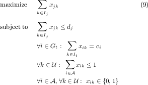
the following way: Given a set of advertisers and their bids,
{(Ii,di,bi)}, find a subset of advertisers, or winners, for which
accepting their bids maximizes the value. This problem is
captured by the following mathematical program. Let yi be the
indicator variable that advertiser i is a winner; zij be the
indicator variable that item j is allocated to advertiser i; and
xi be the total number of items allocated to advertiser
i.
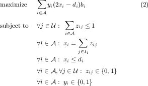
As we show in the next section, it is NP-hard to even approximate the solution of this optimization program within any constant ratio. The main difficulty comes from the multiplicative terms yixi in the objective function of the program above. However, we show that once the set of winning advertisers is determined (i.e., once we fix the {yi} variables), the resulting program can be solved combinatorially using a maximum weighted matching algorithm.
Lemma 2.1. Given the set T of winning advertisers, the problem of finding the optimum allocation of items to advertisers in T can be optimally solved in polynomial time.
 T and yi = 0 otherwise, and by
setting xi = ∑
j
T and yi = 0 otherwise, and by
setting xi = ∑
j Iizij. The negative term in the resulting
objective function is now a constant, and so the problem
reduces to the following program:
Iizij. The negative term in the resulting
objective function is now a constant, and so the problem
reduces to the following program:
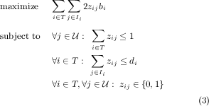
This integer program is equivalent to a maximum weighted
b-matching problem, or f-factor problem, in which, given a
weighted graph G, the goal is to find a maximum-weight subgraph
of G in which the degree of each node i is at most f(i). The
mapping is as follows: consider a bipartite graph G(V,E) with
node set V (G) = ∪ T, edge set E(G) = {(i,j)|i T,j Ii},
and edge weights w(i,j) = 2bi. The solution to the integer
program is then the maximum weighted f-matching in
which f(i) = di for i T and f(j) = 1 for j . We can
therefore use the combinatorial or LP-based algorithms for
f-matching (see, e.g., []west,schrijver,BT98) to solve our
problem. __
The above discussion shows that the challenging part of the banner advertising problem is to decide the set T of winning advertisers.
3. HARDNESS OF APPROXIMATION .
In this section, we show that the banner advertising problem is NP-hard to approximate within any constant ratio. In other words, for any constant 0 < c ≤ 1, it is not possible to find an allocation with value at least c times the optimum value (defined as the value of the mathematical program (2)) in polynomial time unless P = NP.
This result is immediate for arbitrarily large penalties via a reduction from the inapproximable maximum set-packing problem []GJ79, i.e., the problem of finding the maximum number of disjoint sets in a given set family. For arbitrary penalties, we provide a reduction from the k-uniform regular set cover problem. In this problem, we are given a family of sets over a universe of elements. Each set in the family has exactly k elements, and each element in the universe is covered by exactly k sets. The goal is to select the minimum number of sets which cover all the elements. It is shown in Feige et al. []FLT04, Theorem 12, that:
Proposition 3.1. []Feige98, FLT04 For every choice
of constants s0 > 0 and ε > 0, there exists k dependent
on ε and instances of k-uniform regular set cover with n
elements on which it is NP-hard to distinguish between the
case in which all elements can be covered by t =  disjoint
sets, and the case in which every s ≤ s0t sets cover at most
a fraction of 1 - (1 -
disjoint
sets, and the case in which every s ≤ s0t sets cover at most
a fraction of 1 - (1 - )s + ε of the elements.
By introducing an advertiser with bid (Ii,|Ii|, 1) for each set
Ii in the set cover instance, there is a trivial reduction from the
problem above which shows that it is NP-hard to compute the
optimum value of the banner advertising problem. In the case in
which all elements can be covered by t =  disjoint sets, the
optimum value would be n, but, the case in which every
s ≤ s0t sets cover at most a fraction of 1 - (1 -
disjoint sets, the
optimum value would be n, but, the case in which every
s ≤ s0t sets cover at most a fraction of 1 - (1 - )s + ε
of the elements, the optimum value would be less than
n.
)s + ε
of the elements, the optimum value would be less than
n.
In order to prove hardness of approximation, we find an upper bound on the value of the optimum solution in the second case, which leads to the theorem below.
Theorem 3.2. The banner advertising problem is NP-hard to approximate within any constant ratio 0 < c ≤ 1.
The theorem is proved by showing that if one can approximate the solution within a constant ratio, then it is possible to distinguish between the instances of the set cover problem described above. The complete proof is given in appendix A. Although the proof in the appendix is presented assuming the penalty λ is equal to one, the result holds for any constant linear penalty.
In lieu of the above hardness result, we present a greedy heuristic which at each step assigns items to an advertiser that maximizes the profit-per-item. The description of the algorithm is given in Figure 1. Note that it is important to choose an advertiser that maximizes profit-per-item. The example below shows that a naive greedy algorithm which chooses the advertiser with maximum overall profit performs quite poorly even in “easy” instances.
The value that algorithm greedy obtains from the instance in the previous example is equal to the optimum value.
4.1 Performance Guarantee: Bi-Criteria
Approximation
.
We analyze algorithm greedy by developing bi-criteria approximations for our problem. To do so, we compare the value of our solution to the value of the optimal solution with a greater penalty. We say an algorithm is an (α,β)-approximation if it always outputs a solution with value at least β times that of the optimal solution with (larger) penalties α. More formally, an algorithm is an (α,β)-approximation for the problem of selling banner ads if it can always obtains a β fraction of the value of the linear program below – this is the same as LP 2 but with a different objective.
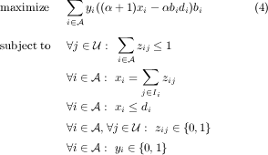
In other words, while our algorithm pays a penalty of 1 for under-allocation, the optimal solution is charged a penalty of α for some α > 1.
For algorithm greedy we can prove the following theorem:
Theorem 4.1. For α ≥ ln 2 __ 1-ln 2 ≈ 2.26, the approximation ratio of greedy algorithm is 1-ln 2 2-ln 2 ≈ 0.23. For 1 < α < ln 2 __ 1-ln 2, the approximation ratio is
where x [ α__
α+1, 1] is the root of the equation 1∕x+(1+1∕α) ln 2x = 2.
be the set
of all advertisers who contribute a positive profit to optα.
For i , let Si be the set optα allocated to advertiser i.
To simplify notation, we use si to denote  . Without loss
of generality, we may assume α __
α+1 < si ≤ 1.
. Without loss
of generality, we may assume α __
α+1 < si ≤ 1.
In the analysis of greedy algorithm, we will partition each item into two subitems: the P subitem that takes up a p fraction of the item, and the Q subitem that takes up a (1 - p) fraction of the item; we will determine the value of p later. We will develop lower bounds on the profit of greedy by a case analysis. In each case, we will compare the profit optα gets to one of two kinds of profit that greedy gets: only to the part computed over P subitems, or only to the part computed over Q subitems. Summing over all advertisers, the P part and Q part of each item, and hence the whole item, is counted at most once.
For i , there are two cases:
When j elements of Si are remaining, greedy could allocate these elements to i with profit-per-item 2j-di____ j bi. This profit is positive for ⌈di∕2⌉ < j ≤|Si|. Therefore, in this case, greedy must have allocated a nonempty set to advertiser i since otherwise greedy could get positive per-item profit by adding i to the solution and allocating the unallocated items of Si to i. Furthermore, as greedy has items of Si available when assigning items to i, it follows that the demand di of advertiser i is fully satisfied. Hence greedy gets complete profit for P subitems, giving a profit of pdibi.
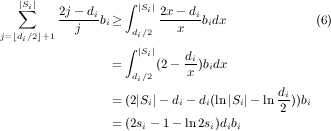
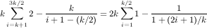
Note, greedy must have obtained a profit of at least 2j-di____ j bi from the (|Si|- j + 1)’th item allocated from Si as this is the per-item profit greedy obtains by allocating the remainder of Si to i. Summing over j, ⌊di∕2⌋ + 1 ≤ j ≤ |Si|, greedy must have allocated these items with total profit at least:
Taking into account that this profit comes only from the Q part of items, this gives a profit of (1 - p)(2si - 1 - ln 2si)dibi.
For each advertiser i, exactly one of the above cases happens. Furthermore, for each item, the P part is counted at most once since the assignment in case 1 is a subset of the solution for greedy and hence disjoint. Similarly, the Q part is also counted at most once since the Si considered in case 2 is a subset of the optimum solution and hence disjoint. Therefore, we have shown that greedy gets a profit of at least:
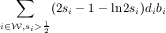
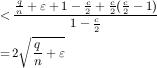
The profit of optα from Si is ((α + 1)si -α)dibi. Therefore, the ratio of the profit of greedy to optα is at least min{p, (1 -p)γ}, where γ is defined as Choosing p = γ __ 1+γ gives the approximation ratio γ __ 1+γ .We find a lower bound on γ using the first and second order conditions. The details of calculations are given in appendix B. For α ≥ ln 2 __ 1-ln 2, γ takes its minimum for si = 1. Plugging in (8), we get γ = 2-1-ln 2 _ (α+1)si-α = 1 - ln 2 and p = 1-ln 2 2-ln 2
For 1 < α < ln 2 __ 1-ln 2, as we prove in appendix B, there exists a point x in [ α__ α+1, 1] for which si = x gives the minimum value of γ. This point is the root of the equation below which is derived by taking the derivatives of (8):

We give an example which shows the analysis is tight for α ≥ ln 2 __ 1-ln 2. In this example, the optimal solution allocates all of the items to the advertisers without paying any penalty. However, the greedy algorithm obtains just a 1-ln 2 2-ln 2 fraction of the optimal solution.
 for each item in row i. He also bids 2 -
 for each
item in column i - k∕2.
for each
item in column i - k∕2.
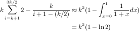
By induction, one can show that at step j, for 1 ≤ j ≤ k∕2, greedy may allocate the top k items in column k - j + 1, to advertiser 3k∕2 -j + 1. Therefore, the total profit of greedy is:
5. AN ADAPTIVE GREEDY ALGORITHM .
As suggested by Example 4.1, fixing the items allocated to each advertiser may hurt the performance of the algorithm. In this section, we give an adaptive greedy algorithm called adaptive greedy. Similar to the previous greedy algorithm, this algorithm iteratively selects new winners. However, in each iteration, it fixes only the number of items assigned to the new winner and not the precise set of items. This flexibility allows adaptive greedy to find the optimum solution in Example 4.1 and, as we will show, allows us to prove better approximation guarantees in general.
We use the following notation throughout this section. For a
winning advertiser i, let ci be the number of items allocated to
i. Note as mentioned above that ci remains fixed although the
set of allocated items may change throughout the course of the
algorithm. Let Gt be the set of advertisers chosen by the
algorithm up to but not including time t. For j Gt, let fjt be
the maximum number of items that we could allocate to
advertiser j, subject to the constraint that each advertiser
i Gt gets exactly ci items. More formally, fjt is the solution of
the following integer program.
Gt, let fjt be
the maximum number of items that we could allocate to
advertiser j, subject to the constraint that each advertiser
i Gt gets exactly ci items. More formally, fjt is the solution of
the following integer program.
Also, let rjt = 2fjt-dj
fjt ⋅ bj be the maximum per-item profit
that we could obtain from advertiser j, subject to the
constraints. At step t, algorithm adaptive greedy chooses the
advertiser with maximum rjt, j Gt. The algorithm is given in
Figure 5.
Gt. The algorithm is given in
Figure 5.
To compute fjt, one can solve the linear relaxation of the above program and round the solution to an integer solution (without decreasing the objective function). For a complete description of the algorithm, we refer the reader to []BT98. 2
5.1 Performance Guarantee: Structural
Approximation
.
As we observed in Section 3, the hardness result implies that we do not hope to analyze the adaptive greedy algorithm by the traditional multiplicative approximation framework. However, in order to distinguish the quality of different algorithms in practice, we can use other approximation measures such as the bi-criteria approximation.
In this section, we analyze the adaptive greedy algorithm using a newly defined framework for evaluating heuristics called structural approximation []FIMN08. The main feature of this framework is that it is designed to evaluate the approximation ratio of an algorithm based on the structure of an optimal (or any) solution, and not only the value of an optimal solution. In this framework, given a solution with some value, we define the recoverable value of the solution based on its structure. The goal is to show that the value of our algorithm is at least as much as the the recoverable value of any solution. 3 We would like to design a recoverable value function that is very close to the real value. Note that in the traditional multiplicative approximation framework, the recoverable value is restricted to a multiplicative ratio of the value of the solution. By allowing more general functions for the recoverable value, the structural approximation framework is more flexible, and therefore can distinguish among different algorithms with the same worst-case multiplicative approximation guarantees. Additionally, this framework provides a way for comparing the quality of our solution to that of the optimal solution of the same problem (with the same parameters). This is in contrast to the bi-criteria approximation framework in which we compare the value of our solution to the value of a problem with different parameters. We refer the reader to []FIMN08 for a more detailed discussion of the structural approximation framework.
We now analyze adaptive greedy algorithm using the
structural approximation framework. Let  be the set of
advertisers that are allocated a non-empty set in the optimal
solution, i.e., the winners. For each advertiser i , let Si be
the set of items allocated to i in an optimal solution. For i ⁄,
Si is taken to be the empty set. Let si = |Si|
di . Then the
value of the optimal solution is: ∑
i
be the set of
advertisers that are allocated a non-empty set in the optimal
solution, i.e., the winners. For each advertiser i , let Si be
the set of items allocated to i in an optimal solution. For i ⁄,
Si is taken to be the empty set. Let si = |Si|
di . Then the
value of the optimal solution is: ∑
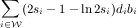
i (2si - 1)dibi. We
define
(2si - 1)dibi. We
define
Theorem 5.1. Let Si be the set of items assigned to advertiser i by an optimal solution. Also, let si = |Si| di . adaptive greedy algorithm obtains a value of at least:
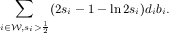
Corollary 5.1. Consider a collection {(qi,αi)} corresponding to an optimal solution, where qi is the fraction of the value of the solution comes from the advertisers for which an αi fraction of the demand is satisfied. Then, the approximation ratio of adaptive greedy is at least:
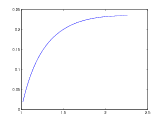
In particular, when in the optimal solution, at least an s fraction of the demand of all winning advertisers is satisfied, adaptive greedy obtains at least a fraction (2s- 1 - ln 2s) of the value of the optimal solution. Figure 4 depicts this lower bound on the value for 1 2 ≤ s ≤ 1.
|
|
 0 be the empty set. The t-th element of the sequence
of assignments, denoted by t, is an assignment of items to
advertisers 1,…,t which satisfies the following properties.
t-1 are also assigned in
t, i.e. are assigned to advertisers 1,…,t.
) are assigned. (This property
trivially holds for i ⁄.)
0 be the empty set. The t-th element of the sequence
of assignments, denoted by t, is an assignment of items to
advertisers 1,…,t which satisfies the following properties.
t-1 are also assigned in
t, i.e. are assigned to advertisers 1,…,t.
) are assigned. (This property
trivially holds for i ⁄.)
In the following lemma, we show that such a sequence of assignments exists.
Lemma 5.1. There exists a sequence {1,2,…,t} of
canonical assignments which satisfies the properties above.
. In
this case we observe that c1 ≥|S1|, and hence a canonical
assignment exists. Therefore, the base of induction holds.
Now consider t > 1. Assume a sequence of canonical
assignments 1,…,t-1, and let t be an optimal solution for
LP (9). We change t to a canonical assignment satisfying
the above three properties. For 1 ≤ i < t, let Bi be the set
of item that are assigned to advertiser i in t-1. Also, let Bt
the set of items in St that are not assigned to any advertiser
in t-1. Note that |Bt|≤ ct, because if we assign each item
in Bi, 1 ≤ i ≤ t, to advertiser i, it gives us a feasible solution
of LP (9).
We repeat the following procedure as long as there exists
an item x such that x Bi, for an advertiser 1 ≤ i ≤ t, and x
is not assigned to any advertisers in t. Since advertiser i has
received ci items in t, and |Bi|≤ ci, there exists an item
y Bi that is assigned to i in t. We update t by assigning
x to i and removing y from the set of items allocated to i.
Note that each time we perform the procedure, the number
of items that is allocated to each advertiser remains the
same. However, the number of items that are allocated to the
same advertisers in t and the assignment defined by Bi’s
increases by 1. Since the number of items that are allocated
to the same advertiser in t and the assignment defined by
Bi’s is at most ∑
1≤i≤tci, after some number of steps, we
reach a point where no such update is possible. Therefore,
the final assignment after these set of updates satisfies all
the three properties. __
Bi that is assigned to i in t. We update t by assigning
x to i and removing y from the set of items allocated to i.
Note that each time we perform the procedure, the number
of items that is allocated to each advertiser remains the
same. However, the number of items that are allocated to the
same advertisers in t and the assignment defined by Bi’s
increases by 1. Since the number of items that are allocated
to the same advertiser in t and the assignment defined by
Bi’s is at most ∑
1≤i≤tci, after some number of steps, we
reach a point where no such update is possible. Therefore,
the final assignment after these set of updates satisfies all
the three properties. __
Now we are ready to prove Theorem 5.1. Note that the value
obtained from each assignment only depends on the number of
items allocated to each advertiser. Therefore, without loss of
generality, we might assume that adaptive greedy allocates to
each advertiser the same set of items assigned to this advertiser
in canonical assignment T.
For i , let kit be the number of items of Si that are not
assigned in t-1. Since we can construct a feasible solution with
value kit for LP (9) using t-1, we observe that fit ≥ kit.
Therefore, the value-per-item that adaptive greedy would
obtain at this point if it chooses advertiser i and assigns to it all
not previously assigned items of Si at least (2 - di _
kit)bi. Thus,
the value adaptive greedy obtains by the end of the
algorithm is at least:
For i , if advertiser i is chosen by adaptive greedy then
kiT = 0, and if advertiser i is not chosen by adaptive greedy
then necessarily kiT ≤ di
2 . Therefore:
By the same calculation as in Theorem 4.1, equation (6), the value obtained by adaptive greedy is at least:
Note that while we stated all our results with respect to the recoverable value of an optimal solution, our proofs in fact follow when considering the recoverable value of any solution.
5.2 Comparison of GREEDY and ADAPTIVE GREEDY .
We analyzed adaptive greedy algorithm using the structural approximation framework. We also analyzed the greedy algorithm using the bi-criteria approximation framework. In order the compare these two greedy algorithms, we now analyze the greedy algorithm in the structural approximation framework.
Let be the set of the winners in an optimum solution (or
any feasible solution). Assume that this solution satisfies a si
fraction of the demand of advertiser i . Note that si ≥ 1
2,
i . By equation (7), in the proof of Theorem 4.1,
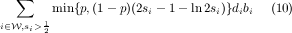
for any p, 0 ≤ p ≤ 1, greedy obtains a value of at least:
Given si’s, one can compute the value of p which maximizes the sum and gives a recoverable value for each solution. However, by Theorem 5.1, the value of adaptive greedy algorithm from the same instance is at least:
This immediately shows that adaptive greedy gives us a better guarantee on the value of the solution.
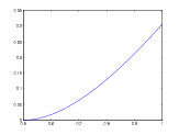
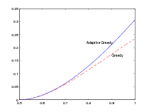
When in an optimum solution, fraction s of the demand of all advertisers is satisfied, we can easily compare the guarantees on the value given in Theorems 4.1 and 5.1. In this case, the optimum value for p in (10) is equal to 2s-1-ln 2s 2s-ln 2s , which leads to the same guarantee on the approximation ratio of greedy algorithm. The guarantee on the approximation ratio of adaptive greedy algorithm is 2s - 1 - ln 2s. Figure 5 depicts these guarantees on the approximation ratio for 1_ 2 ≤ s ≤ 1.
|
|
One way to see that adaptive greedy strictly outperforms greedy is to observe that adaptive greedy algorithm obtains the optimum value of the instance described in Example 4.1. As a result, the ratio between the values of the solutions obtained by these two algorithms is 2 - ln 2.
In this paper we showed that having supply guarantees makes the problem of maximizing the value of selling banner advertisements inapproximable. In the lieu of this hardness result, we proposed two greedy heuristics for the banner advertising problem and analyzed them rigorously in the bi-criteria and structural approximation frameworks. Given the simple and flexible nature of these algorithms, we expect that these algorithms can help in automating the negotiation process for banner advertising.
In order to make our algorithms even more applicable to practical settings, we would like to consider the online or stochastic settings, in which advertisers arrive over time and submit bids which must be immediately accepted or rejected, without knowledge of exact future demand. Also along these lines, it would also be useful to relax the assumption that the supply of items is known a priori. In practice, hosts have good estimates of the number of page views. However, these estimates may have large variance, and we should ideally provide algorithms which are robust with respect to errors in the supply estimates. Finally, to completely automate the banner advertising process and replace it with a repeated auction mechanism, it is necessary to design a pricing mechanism to accompany our allocation mechanism and analyze the resulting incentives.
APPENDIX
A. PROOF OF THEOREM 3.2
. Proof. We prove that claim holds even if the advertisers
have large demands. We define a special case of selling
banner advertisements . Consider m sets A1, ,Am, each
of size k; let A = ∪i=1mA
i and n = |A|. Also consider a set
Q of size q which is disjoint from A. Also, assume k = O(q)
and kq = o(
,Am, each
of size k; let A = ∪i=1mA
i and n = |A|. Also consider a set
Q of size q which is disjoint from A. Also, assume k = O(q)
and kq = o( ).
).
Problem  (k,q,n) is defined with m advertisers. Let
c = 2(1 -
(k,q,n) is defined with m advertisers. Let
c = 2(1 - ). Let the bid of advertiser i, (Ii,di,bi),
be equal to (Q ∪ Ai,ck, 1). We show that it is NP-Hard to
approximate (k,q,n) within a ratio of 2
). Let the bid of advertiser i, (Ii,di,bi),
be equal to (Q ∪ Ai,ck, 1). We show that it is NP-Hard to
approximate (k,q,n) within a ratio of 2 .
.
Consider the k-uniform regular set cover instances
defined in the proposition 3.1, for ε and s0 = 3. We say an
instance is of type YES if all elements can be covered by
t disjoint sets. An instance is of type NO if every s ≤ s0t
sets cover at most a fraction of 1 - (1 - )s + ε of the
elements. We show if an algorithm can approximate problem
(k,q,n) within a ratio of 2
)s + ε of the
elements. We show if an algorithm can approximate problem
(k,q,n) within a ratio of 2 , then this algorithm can
distinguishes between YES and NO instances.
, then this algorithm can
distinguishes between YES and NO instances.
For the YES instances, there are t =  disjoint set which
cover all the n elements. Hence, the value in this case is at
least t(k - (kc - k)) = n(2 - c).
disjoint set which
cover all the n elements. Hence, the value in this case is at
least t(k - (kc - k)) = n(2 - c).
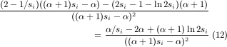
For a NO instance, any s sets, 0 ≤ s ≤ s0t, cover at most
q + (1 - (1 - )s + ε)n elements. Therefore, the value of any s
sets is at most 2(q + (1 - (1 -
)s + ε)n elements. Therefore, the value of any s
sets is at most 2(q + (1 - (1 - )s + ε)n) -csk. Note that t can
be made arbitrary large ([]FLT04); hence, we can approximate
(1 -
)s + ε)n) -csk. Note that t can
be made arbitrary large ([]FLT04); hence, we can approximate
(1 - ) with e
 with arbitrary accuracy. Thus, the value of
any s sets is at most:
with arbitrary accuracy. Thus, the value of
any s sets is at most:
We find the optimum value for s by the first order conditions:

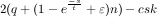
Plugging s = -t log  in (11), the maximum value is at most
2(q + (1 -
in (11), the maximum value is at most
2(q + (1 - + ε)n) + cn log
  . Note that the value for any choice
of m ≥ s0t sets is negative, because the total demand is more
than double of the number of elements. Therefore, the ratio
between the value from a NO instance and a Yes instance is at
most:
. Note that the value for any choice
of m ≥ s0t sets is negative, because the total demand is more
than double of the number of elements. Therefore, the ratio
between the value from a NO instance and a Yes instance is at
most:
Recall that 1 - =
=  , which completes the proof. __
B. FINDING A LOWER BOUND ON γ .
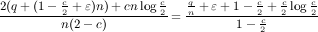
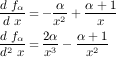
Here, we compute a lower bound on the value of γ defined in (8). Taking the derivative of 2si-1-ln 2si (α+1)si-α with respect to si:
Define fα(x) = α∕x - 2α + (α + 1) ln 2x,x (0, 1]. The first
and the second derivative of fα with respect to x are:
Hence, for α > 1 and x (0, 1], function fα is strictly convex
and takes its minimum at x = α __
α+1. Therefore, fα is increasing
in [ α__
α+1, 1].
If fα(1) = ln 2 - (1 - ln 2)α ≤ 0, then fα is negative in [ α__ α+1, 1]. Hence, (12) is decreasing in [ α__ α+1, 1], and take its minimum at 1. For α ≥ ln 2 __ 1-ln 2, fα(1) ≤ 0. Plugging in (8), γ = 2-1-ln 2 _ (α+1)si-α = 1 - ln 2. Therefore, for this range of α, the approximation ratio is 1-ln 2 2-ln 2.
For 1 < α < ln 2 __ 1-ln 2, as we prove later, fα( α__ α+1) is negative. Because fα(1) is positive, by the intermediate value theorem, there exists a point x* in [ α__ α+1, 1] for which fα is zero. This point is the root of equation:

Because fα is increasing in [ α__ α+1, 1], by convexity, x* gives the minimum value of (12). Plugging this value for γ into γ __ 1+γ , we get (5) as a lower bound on the approximation ratio of 1 < α < ln 2 __ 1-ln 2.
Now we only need to show that for α > 1, fα( α__ α+1) is negative. For x = 1 2, fα(1 2) = 2α - 2α + (α + 1) ln 1 = 0. Also, fα is strictly convex and takes its minimum at α __ α+1 > 1 2. Therefore, fα( α__ α+1) < 0.