 |
1
Qiaozhu Mei, Deng Cai, Duo Zhang, ChengXiang Zhai
Department of Computer Science
University of Illinois at Urbana-Champaign
In this paper, we formally define the problem of topic modeling with network structure (TMN). We propose a novel solution to this problem, which regularizes a statistical topic model with a harmonic regularizer based on a graph structure in the data. The proposed method combines topic modeling and social network analysis, and leverages the power of both statistical topic models and discrete regularization. The output of this model can summarize well topics in text, map a topic onto the network, and discover topical communities. With appropriate instantiations of the topic model and the graph-based regularizer, our model can be applied to a wide range of text mining problems such as author-topic analysis, community discovery, and spatial text mining. Empirical experiments on two data sets with different genres show that our approach is effective and outperforms both text-oriented methods and network-oriented methods alone. The proposed model is general; it can be applied to any text collections with a mixture of topics and an associated network structure.
Categories and Subject Descriptors: H.3.3 [Information
Search and Retrieval]: Text Mining
General Terms: Algorithms
Keywords: statistical topic models, social networks,
graph-based regularization
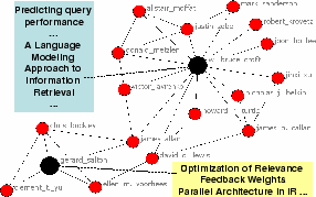
With the prevailing of Web 2.0 applications, more and more web users are actively publishing text information online. These users also often form social networks in various ways, leading to simultaneous growth of both text information and network structures such as social networks. Taking weblogs (i.e., blogs) as an example, one can find a wide coverage of topics and diversified discussions in the blog posts, as well as a fast evolving friendship network among the bloggers. In another scenario, as researchers are regularly publishing papers, we not only obtain text information, but also naturally have available co-authorship networks of authors. In yet another scenario, as email users produce many text messages, they also form networks through the relation of sending or replying to messages. One can easily imagine many other examples of text accompanied by network structures such as webpages accompanied by links and literature accompanied by citations. Figure 1 presents an example coauthor network from SIGIR proceedings, where each author is associated with the papers he/she published.
These examples show that in many web mining tasks, we are often dealing with collections of text with a network structure attached, making it interesting to study how we can leverage the associated network structure to discover interesting topic and/or network patterns.
Statistical topic models have recently been successfully applied to multiple text mining tasks [10,4,28,26,20,15,27] to discover a number of topics from text. Some recent work has incorporated into topic modeling context information [20], such as time [27], geographic location [19], and authorship [26,23,19], to facilitate contextual text mining. Topics discovered in this way can be used to infer research communities [26,23] or information diffusion over geographic locations [19]. However, they do not consider the natural network structure among authors, or geographic locations. Intuitively, these network structures are quite useful for refining and structuring topics, and are sometimes essential for discovering network-associated topics. For example, two researchers who often coauthor with each other are likely to be working on the same topics, thus are likely to be in the same research community. For geographically sensitive events (e.g., hurricane Katrina), bloggers living at adjacent locations tend to write about similar topics. The lack of consideration of network structures is also a deficiency in some other text mining techniques such as document clustering.
On the other hand, social network analysis (SNA) focuses on the topology structure of a network [11,13,1,12], addressing questions such as ``what the diameter of a network is [13]'', ``how a network evolves [13,1]'', ``how information diffuses on the network [9,14]'', and ``what are the communities on a network [11,1].'' However, these techniques usually do not leverage the rich text information. In many scenarios, text information is very helpful for SNA tasks. For example, Newton and Einstein had never collaborated on a paper (i.e., social network), but we still consider them in the same research (physics) community because they made research contributions on related research topics (i.e., text). Similarly, to attract Bruce Willis to take a role in a movie, ``the script is interesting (i.e., text)'' is as important as ``the director is a trustable friend (i.e., social network).''
Is there a way to leverage the power of both the textual topics and the network structure in text mining? Can the two successful complementary mining techniques (i.e., probabilistic topic modeling and social network analysis) be combined to help each other? To the best of our knowledge, these questions have never been seriously studied before. As a result, there is no principled way to combine the mining process of topics in text and social networks (e.g., combining topic modeling with network analysis). Although methods have been proposed to combine page contents and links in web search [22], none of them is tuned for text mining.
In this paper, we formally define the major tasks of Topic Modeling with Network Structure (TMN), and propose a unified framework to combine statistical topic modeling with network analysis by regularizing the topic model with a discrete regularizer defined based on the network structure. The framework makes it possible to cast our mining problem as an optimization problem with an explicit objective function. Experiment results on different genres of real world data show that our model can effectively extract topics, generat topic maps on a network, and discover topical communities. The results also show that our model improves over both pure text mining methods and pure network analysis methods, suggesting the necessity of combining them.
The proposed framework of regularized topic modeling is general; one can choose any topic model and a corresponding regularizer on the network. Variations of the general model are effective for solving real world text mining problems, such as author-topic analysis and spatial topic analysis.
The rest of this paper is organized as follows. In Section 2, we formally define the problem of topic modeling with network structure. In Section 3, we propose the unified regularization framework as well as two general methods to solve the optimization problem. We discuss the variations and applications of our model in Section 4 and present empirical experiments in Section 5. Finally, we discuss the related work in Section 6 and conclude in Section 7.
We assume that the data to be analyzed consists of both a collection of text documents and an associated network structure. This setup is quite general: The text documents can be a set of web pages, blog articles, scientific literature, emails, or profiles of web users. The network structure can be any social networks on the web, co-author/citation graphs, geographic networks, or even latent networks that can be inferred from the text (e.g., entity-relation graph, document nearest-neighbor graph, etc). We now formally define the related concepts and the general tasks of topic modeling with network structure.
Definition 1 (Document): A text document
![]() in a text collection
in a text collection
![]() is a sequence of words
is a sequence of words
![]() , where
, where
![]() is a word from a fixed
vocabulary. Following a common simplification in most work in
information retrieval and topic modeling [10,4], we represent a document with a
bag of words, i.e.,
is a word from a fixed
vocabulary. Following a common simplification in most work in
information retrieval and topic modeling [10,4], we represent a document with a
bag of words, i.e.,
![]() . We use
. We use
![]() to denote the occurrences
of word
to denote the occurrences
of word ![]() in
in ![]() .
.
Definition 2 (Network): A network
associated with a text collection ![]() is a graph
is a graph
![]() , where
, where
![]() is a set of vertices and
is a set of vertices and
![]() is a set of edges. Without
losing generality, we define a vertex
is a set of edges. Without
losing generality, we define a vertex ![]() as a subset of documents
as a subset of documents
![]() . For
example, a vertex in a coauthor graph can be a single author
associated with all papers he/she published. An
edge
. For
example, a vertex in a coauthor graph can be a single author
associated with all papers he/she published. An
edge
![]() is a binary
relation between vertices
is a binary
relation between vertices ![]() and
and
![]() , where we use
, where we use ![]() to denote the weight of
to denote the weight of
![]() . An edge can
be either undirected or directed. In this work, we
only consider the undirected case, i.e.,
. An edge can
be either undirected or directed. In this work, we
only consider the undirected case, i.e.,
![]() .
.
Definition 3 (Topic): A semantically coherent
topic in a text collection ![]() is represented by a topic model
is represented by a topic model
![]() , which is a
probabilistic distribution of words
, which is a
probabilistic distribution of words
![]() .
Clearly, we have
.
Clearly, we have
![]() . We assume that there are
all together
. We assume that there are
all together ![]() topics in
topics in ![]() .
.
By combining text topics and a network structure, we can discover new types of interesting patterns. For example, we can explore who first brought the topic ``language modeling'' into the IR community, and who have been diffusing this topic on the research network. A topic could also define a latent community on the network (e.g., the machine learning community, the SNA community, etc). The following patterns are unique to topic modeling with network structure, and cannot be discovered solely from text or social networks.
Definition 4 (Topic Map): A topic map of
a topic ![]() on network
on network
![]() ,
, ![]() , is represented by a vector of weights
, is represented by a vector of weights
![]() ,
where
,
where ![]() , and
, and ![]() is a weighting function of a topic on a
vertex. For example, we may define
is a weighting function of a topic on a
vertex. For example, we may define ![]() as
as
![]() , where
, where
![]() for all
for all ![]() . From a topic map, we can
learn how a topic is distributed on the network. Intuitively, we
expect that the adjacent vertices be associated with similar
topics and the weights of topics on adjacent vertices are
similar.
. From a topic map, we can
learn how a topic is distributed on the network. Intuitively, we
expect that the adjacent vertices be associated with similar
topics and the weights of topics on adjacent vertices are
similar.
Definition 5 (Topical Community): A topical
community on network ![]() is
represented by a subset of vertices
is
represented by a subset of vertices
![]() . We
can assign a vertex
. We
can assign a vertex ![]() to
to
![]() with any
reasonable criterion, e.g.
with any
reasonable criterion, e.g.
![]() , or
, or
![]() . The
topic model
. The
topic model ![]() is then a natural
summary of the semantics of the topical community
is then a natural
summary of the semantics of the topical community
![]() . Intuitively we
expect that the vertices within the same topical community are
tightly connected and all have a large
. Intuitively we
expect that the vertices within the same topical community are
tightly connected and all have a large ![]() ; vertices from different topical communities
are loosely connected and have different
; vertices from different topical communities
are loosely connected and have different ![]() . A topical community is different from
a community in the SNA literature in that it must have
coherent semantics, and can be summarized with a coherent
topic in text.
. A topical community is different from
a community in the SNA literature in that it must have
coherent semantics, and can be summarized with a coherent
topic in text.
Based on the definitions of these concepts, we can formalize the major tasks of topic modeling with network structure (TMN) as follows:
Task 1: (Topic Extraction) Given a collection
![]() and a network structure
and a network structure
![]() , the task of Topic
Extraction is to model and extract
, the task of Topic
Extraction is to model and extract ![]() major topic models,
major topic models,
![]() ,
where
,
where ![]() is a user specified
parameter.
is a user specified
parameter.
Task 2: (Topic Map Extraction) Given a collection
![]() and a network structure
and a network structure
![]() , the task of Topic Map
Extraction is to model and extract the
, the task of Topic Map
Extraction is to model and extract the ![]() weight vectors
weight vectors
![]() , where each vector
, where each vector
![]() is a map of topic
is a map of topic
![]() on network
on network ![]() .
.
Task 3: (Topical Community Discovery) Given a
collection ![]() and a network
structure
and a network
structure ![]() , the task of Topical
Community Discovery is to extract
, the task of Topical
Community Discovery is to extract ![]() topical communities
topical communities
![]() , where each
, where each
![]() has a coherent
semantic summary
has a coherent
semantic summary ![]() , which
is one of the
, which
is one of the ![]() major topics in
major topics in
![]() .
.
These tasks are challenging in many ways. First, there is no existing unified model that can embed a network structure in a topic model. Indeed, whether a social network structure can help extracting topics is an open question. Second, in existing community discovery methods, there is no guarantee that the semantics of a community is coherent. It is rather unclear how to satisfy the topical coherency and the connectivity coherency at the same time. Moreover, since it is usually hard to create training examples to this problem, the solution has to be unsupervised.
The three major tasks above are by no means the only tasks of topic modeling with network structure. With the output of such basic tasks, more in-depth analysis can be done. For example, one can compare topic maps over time and analyze how topics are propagating over the network. One can also track the evolution of topical communities.
In this section, we propose a novel and general framework of regularizing statistical topic models with the network structure.
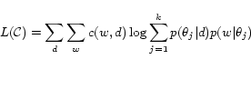
We first discuss the basic statistical topic models, which
have been applied to many text mining tasks [10,4,26,19,15,27,20]. The basic idea of these models
is to model documents with a finite mixture model of ![]() topics and estimate the model
parameters by fitting the data with the model. Two basic
statistical topic models are the Probabilistic Latent Semantic
Analysis (PLSA) [10] and
the Latent Dirichlet Allocation (LDA) [4]. For example, the log likelihood
of a collection
topics and estimate the model
parameters by fitting the data with the model. Two basic
statistical topic models are the Probabilistic Latent Semantic
Analysis (PLSA) [10] and
the Latent Dirichlet Allocation (LDA) [4]. For example, the log likelihood
of a collection ![]() to be
generated with PLSA is given as follows:
to be
generated with PLSA is given as follows:
The parameters in PLSA are
![]() .
Naturally, we can use
.
Naturally, we can use
![]() as the
weights of topics on vertex
as the
weights of topics on vertex ![]() , and
compute
, and
compute ![]() by
by
 |
(2) |
PLSA thus provides an over-simplified solution to the problem
of TMN by ignoring the network structure. There is no guarantee
that vertices in the same topical community are well connected,
or adjacent vertices are associated with similar topics. Indeed,
a limitation of PLSA is that there is no constraint on the
parameters
![]() for
different
for
different ![]() , the number of which grows
linearly with the data. Therefore, the parameters
, the number of which grows
linearly with the data. Therefore, the parameters
![]() would overfit the data. To alleviate this overfitting problem,
LDA assumes that the document-topic distributions
would overfit the data. To alleviate this overfitting problem,
LDA assumes that the document-topic distributions
![]() of
each document
of
each document ![]() are all generated from
the same Dirichlet distribution.
are all generated from
the same Dirichlet distribution.
We propose a new framework to model topics with a network
structure, by regularizing a statistical topic model with a
regularizer on the network. The criterion of this regularization
is succinct and natural: vertices which are connected to each
other should have similar weights of topics (
![]() ).
).
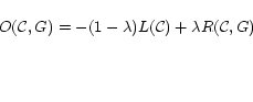
Formally, we define a regularized data likelihood as
This regularization framework is quite general. We can use any
statistical topic model to refine ![]() , and use any graph based regularizer
, and use any graph based regularizer
![]() as long as it can
smooth the topics among adjacent vertices. We abbreviate the
network regularized statistical topic model as NetSTM.
as long as it can
smooth the topics among adjacent vertices. We abbreviate the
network regularized statistical topic model as NetSTM.
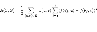
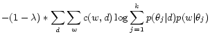
To illustrate this framework, in this paper we use PLSA as the
statistical topic model and a regularizer similar to the graph
harmonic function in [33],
i.e.,
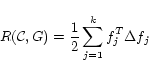
Note that the regularizer in Equation 4
is an extension of the graph harmonic function in [33] to multiple classes (topics). It
can be rewritten as
 |
(5) |
This framework is a general one that can leverage the power of
both the topic model and the graph Laplacian regularization.
Intuitively, the ![]() in
Equation 6 measures how likely the data is
generated from this topic model. By minimizing
in
Equation 6 measures how likely the data is
generated from this topic model. By minimizing ![]() , we will find
, we will find
![]() and
and
![]() which fits
the text data as much as possible. By minimizing
which fits
the text data as much as possible. By minimizing ![]() , we smooth the topic distributions on the
network structure, where adjacent vertices have similar topic
distributions.
, we smooth the topic distributions on the
network structure, where adjacent vertices have similar topic
distributions.
Although theoretically ![]() can be defined as any weighting function of a
topic
can be defined as any weighting function of a
topic ![]() on
on ![]() , in practice it must be a function of the parameters
in PLSA (i.e.,
, in practice it must be a function of the parameters
in PLSA (i.e.,
![]() and
and
![]() ). When a
vertex have multiple documents, an example choice is
). When a
vertex have multiple documents, an example choice is
![]() .
.
The parameter ![]() can then
be set between 0 to 1 to control the balance between the data
likelihood and the smoothness of topic distributions over the
network. It is easy to show that if
can then
be set between 0 to 1 to control the balance between the data
likelihood and the smoothness of topic distributions over the
network. It is easy to show that if ![]() , the objective function boils down to the log
likelihood of PLSA. Minimizing
, the objective function boils down to the log
likelihood of PLSA. Minimizing
![]() will give us the
topics which best fit the content of the collection. When
will give us the
topics which best fit the content of the collection. When
![]() , this objective
function boils down to
, this objective
function boils down to
![]() . Embedded with
additional constraints, this is related to the objective of
spectral clustering (i.e., ratio cut [6]). By minimizing
. Embedded with
additional constraints, this is related to the objective of
spectral clustering (i.e., ratio cut [6]). By minimizing
![]() , we will extract
document clusters solely based on the network structure.
, we will extract
document clusters solely based on the network structure.
An interesting simplified case is when every vertex only
contains one document (thus substitute ![]() ,
, ![]() with
with ![]() ,
, ![]() ) and
) and
![]() . Then we have
. Then we have
Let us first consider the special case when ![]() . In such a case, the objective function
degenerates to the log-likelihood function of PLSA with no
regularization.
. In such a case, the objective function
degenerates to the log-likelihood function of PLSA with no
regularization.
The standard way of parameter estimation for PLSA is to apply
the Expectation Maximization (EM) algorithm [8] which iteratively computes a
local maximum of ![]() .
Specifically, in the E-step, it computes the expectation of the
complete likelihood
.
Specifically, in the E-step, it computes the expectation of the
complete likelihood
![]() , where
, where
![]() denotes all the parameters,
and
denotes all the parameters,
and ![]() denotes the value of
denotes the value of
![]() estimated in the last
(
estimated in the last
(![]() -th) EM iteration. In the
M-step, the algorithm finds a better estimate of parameters,
-th) EM iteration. In the
M-step, the algorithm finds a better estimate of parameters,
![]() , by maximizing
, by maximizing
![]() :
:
Computationally, the E-step boils down to computing the
conditional distribution of the hidden variables given the data
and ![]() . The hidden variables in
PLSA correspond to the events that a term
. The hidden variables in
PLSA correspond to the events that a term ![]() in document
in document ![]() is generated
from the
is generated
from the ![]() -th topic. Formally, we
have the E-Step:
-th topic. Formally, we
have the E-Step:
| (9) |
The maximization problem in the M-Step (i.e., Equation
7) has a closed form solution:
We now discuss how we can extend this standard EM algorithm to
handle the case
![]() . Using a similar
derivation to that of the EM algorithm, we have the following
expected complete likelihood function for NetPLSA, where for
convenience of discussion, we also added the Lagrange multipliers
corresponding to the constraints on our parameters:
. Using a similar
derivation to that of the EM algorithm, we have the following
expected complete likelihood function for NetPLSA, where for
convenience of discussion, we also added the Lagrange multipliers
corresponding to the constraints on our parameters:
where
![]() and
and
![]() are Lagrange
multipliers corresponding to the constraints that
are Lagrange
multipliers corresponding to the constraints that
![]() and
and
![]() .
.
Thus in general, we can still use the EM algorithm to estimate
the parameters when ![]() in Equation 6 by maximizing
in Equation 6 by maximizing
![]() . It is easy to
see that NetPLSA shares the same hidden variables with PLSA, and
the conditional distribution of the hidden variables can still be
computed using Equation 8. Thus the
E-step remains the same.
. It is easy to
see that NetPLSA shares the same hidden variables with PLSA, and
the conditional distribution of the hidden variables can still be
computed using Equation 8. Thus the
E-step remains the same.
The M-step is more complicated due to the introduction of the
regularizer. The estimation of ![]() does not rely on the regularizer, thus
can still be computed using Equation 10. Unfortunately, we do not have a closed
form solution to re-estimate the parameters
does not rely on the regularizer, thus
can still be computed using Equation 10. Unfortunately, we do not have a closed
form solution to re-estimate the parameters
![]() through maximizing
through maximizing
![]() .
.
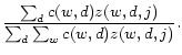
To solve this problem, we can apply a Newton-Raphson method to
update ![]() by finding a local
maximum of
by finding a local
maximum of
![]() in the M step.
Specifically, let
in the M step.
Specifically, let ![]() be the vector
of variables to be updated with the Newton-Raphson method (i.e.,
be the vector
of variables to be updated with the Newton-Raphson method (i.e.,
![]() and
and
![]() ). The updating
formula of the Newton-Raphson's method is as follows:
). The updating
formula of the Newton-Raphson's method is as follows:
| (14) |
We want to set the start point of ![]() corresponding to
corresponding to ![]() . This is because, to guarantee that the generalized
EM algorithm will converge, we need to assure
. This is because, to guarantee that the generalized
EM algorithm will converge, we need to assure
![]() . By setting
the start point of Newton-Raphson method at
. By setting
the start point of Newton-Raphson method at ![]() , we ensure that
, we ensure that ![]() would not drop.
would not drop.
In the previous section, we give a way to gradually approach
the local maximum of
![]() at M step.
However, this involves multiple iterations of Newton-Raphson
updating, in each of which we need to solve a linear system of
at M step.
However, this involves multiple iterations of Newton-Raphson
updating, in each of which we need to solve a linear system of
![]() variables. This significantly increases the cost of parameter
estimation of NetPLSA.
variables. This significantly increases the cost of parameter
estimation of NetPLSA.
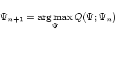
In this section, we propose a simpler algorithm for parameter
estimation based on the generalized EM algorithm (GEM) [21]. According to GEM, we do not
have to find the local maximum of
![]() at every
M step; instead, we only need to find a better value of
at every
M step; instead, we only need to find a better value of
![]() in the M-step, i.e., to
ensure
in the M-step, i.e., to
ensure
![]() .
.
Thus our idea is to optimize the likelihood part and the
regularizer part of the objective function separately in hope of
finding an improvement of the current ![]() . Specifically, let us write
. Specifically, let us write
![]() ,
where
,
where ![]() denotes the
expectation of the complete likelihood of the topic model.
Clearly,
denotes the
expectation of the complete likelihood of the topic model.
Clearly,
![]() holds if
holds if
![]() . We introduce
. We introduce
![]() ,
which is the first eligible set of parameter values that assure
,
which is the first eligible set of parameter values that assure
![]() .
.
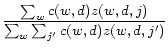
At every M-step, we would first attempt to find
![]() to maximize
to maximize
![]() instead of the
whole
instead of the
whole
![]() . This can be
done by simply applying Equation 11
and 10. Clearly,
. This can be
done by simply applying Equation 11
and 10. Clearly,
![]() does
not necessarily hold as the regularizer part may have been
decreased. Thus we further start from
does
not necessarily hold as the regularizer part may have been
decreased. Thus we further start from
![]() and attempt to
increase
and attempt to
increase
![]() .
.
The Hessian matrix of
![]() is the graph
Laplacian matrix (i.e.,
is the graph
Laplacian matrix (i.e.,
![]() ). By applying one
Newton-Raphson step on
). By applying one
Newton-Raphson step on ![]() ,
we propose a closed form solution for
,
we propose a closed form solution for
![]() ; we then
repeatedly obtain
; we then
repeatedly obtain
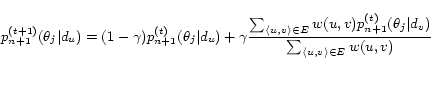
![]() , ...,
, ...,
![]() using the
Equation 15 until the value of the
Q-function starts to drop:
using the
Equation 15 until the value of the
Q-function starts to drop:
Clearly,
![]() and
and
![]() always hold in
Equation 15. When the step parameter
always hold in
Equation 15. When the step parameter
![]() is set to 1, it means
that the new topic distribution of a document is the average of
the old distributions from its neighbors. This is related to the
random-walk interpretation in [33]. Every iteration of Equation
15 makes the topic distributions
smoother on the network. Note that an inner iteration does not
affect the estimation of
is set to 1, it means
that the new topic distribution of a document is the average of
the old distributions from its neighbors. This is related to the
random-walk interpretation in [33]. Every iteration of Equation
15 makes the topic distributions
smoother on the network. Note that an inner iteration does not
affect the estimation of
![]() in
in
![]() .
.
The stepping parameter ![]() can be interpreted as a controlling factor of smoothing the topic
distribution among the neighbors. Once we have found
can be interpreted as a controlling factor of smoothing the topic
distribution among the neighbors. Once we have found
![]() , we can
limit the further iterations of processing of Equation 15, so that
, we can
limit the further iterations of processing of Equation 15, so that ![]() would not be too far away from
would not be too far away from
![]() .
.
The framework defined in Equation 3
is quite general. Actually, one can use any topic models for
![]() and a related
regularizer for
and a related
regularizer for
![]() . The choice of
the topic model and the regularizer should be task dependent. In
this section, we show that with difference choices of
. The choice of
the topic model and the regularizer should be task dependent. In
this section, we show that with difference choices of ![]() and
and ![]() , this framework can be applied to different mining
tasks.
, this framework can be applied to different mining
tasks.
Author-topic analysis has been proposed in text mining
literature [26,23,20]. One major task of author-topic
analysis is to extract research topics from scientific literature
and to measure the associations between topics and authors. This
can be regarded as modeling topic maps and discovering research
communities solely based on textual contents, where the authors
in the same community works on the same topic. With a topic
model, one can find a summary for a topical community, e.g.,
using the distribution ![]() .
.
On the other hand, many methods have been proposed to discover communities from social networks [11,1], which solely explore the network structure. One concrete example is to discover research communities based on the coauthor relationship between researchers, where authors with collaborations are likely to lie in the same community.
However, both directions have their own limitations. In author-topic analysis, the associations between authors are indirectly modeled through the content. A professor and his fellow student may be assigned to two different communities, if they have different flavor of topics. On the other hand, solely relying on the network structure is at risk of assigning a biologist and a computer scientist into the same community, even if they just coauthored one paper of bioinformatics. Moreover, it is difficult to summarize the semantics of a community (i.e., to explain why they form a community).
To leverage the information in the text and the network, we
can apply the NetPLSA model to extract topical communities.
Specifically, for each author ![]() , we
may concatenate all his/her publications to form a virtual
document of
, we
may concatenate all his/her publications to form a virtual
document of ![]() . Then a coauthor social
network
. Then a coauthor social
network ![]() is constructed where there
is an edge between author
is constructed where there
is an edge between author ![]() and
and
![]() if they coauthored at least
one paper.
if they coauthored at least
one paper.
We can define ![]() as the
number of papers that
as the
number of papers that ![]() and
and
![]() coauthored. Equation
6 can be rewritten as
coauthored. Equation
6 can be rewritten as
By minimizing
![]() , we can estimate
, we can estimate
![]() , which
denotes the probability that the author
, which
denotes the probability that the author ![]() belongs to the
belongs to the ![]() -th
topical community. The estimated distribution
-th
topical community. The estimated distribution ![]() can be used as a semantic summary of
the
can be used as a semantic summary of
the ![]() -th community.
-th community.
A general task in spatial text mining [20] is to extract topics from text with location labels and model their distribution over different geographic locations. Some natural topics, like public reaction to an event (e.g., hurricane Katrina), are geographic correlated. Intuitively we can expect that people live at nearby locations express similar topics.
Let ![]() be a set of geographic
locations and
be a set of geographic
locations and ![]() . We denote
. We denote
![]() if document
if document
![]() has a location label of
has a location label of
![]() . By introducing a vertex for
every location and an edge between two adjacent locations, we
construct a geographic location network
. By introducing a vertex for
every location and an edge between two adjacent locations, we
construct a geographic location network
![]() . We can
then model the geographic topic distribution with a variation of
the NetPLSA, where
. We can
then model the geographic topic distribution with a variation of
the NetPLSA, where
We then use the following formula instead of Equation 15:
where ![]() denotes the location
which
denotes the location
which ![]() belongs to.
belongs to.
In the previous sections, we introduced the novel framework of
topic modeling with network regularization, and discussed how it
could be applied to solve real world text mining problems. In
this section, we show the effectiveness of our model with
experiments on two genres of data. We show how NetPLSA works for
the author-topic analysis in Section ![]() and for spatial topic analysis in Section
and for spatial topic analysis in Section ![]() .
.
The Digital Bibliography and Library Project (DBLP) is a
database which contains the basic bibliographic information of
computer science publications 2. In this experiment, we create
our testing data set (4-CONF) from a subset of the DBLP records.
We first extract all the papers published at four different
conferences, WWW, SIGIR, KDD, and NIPS. For each paper, we
extract the title in text and all its authors. We then construct
the coauthor network, by making a vertex for every unique author
![]() and an edge
and an edge
![]() between
two authors if they have coauthored at least one paper. We weight
each edge in this network, by the number of papers that the two
researchers have coauthored,
between
two authors if they have coauthored at least one paper. We weight
each edge in this network, by the number of papers that the two
researchers have coauthored, ![]() . Finally, we concatenate the titles of all papers
of an author to create a document
. Finally, we concatenate the titles of all papers
of an author to create a document ![]() associated with this author. Our dataset has 9041
authors, and 16902 unique edges (without self links); the average
weight for an edge is 1.2.
associated with this author. Our dataset has 9041
authors, and 16902 unique edges (without self links); the average
weight for an edge is 1.2.
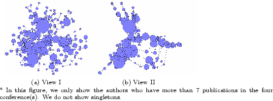
In Figure 2, we visualize the coauthor network structure of the 4-CONF dataset using the NetDraw software3. We only show the authors with more than five publications. The two views are ``Spring Embedder'' and ``Gower Metric Scaling'' provided by NetDarw. Basically, Spring Embedder is a standard graph layout algorithm which tries to put two vertices which are connected by an edge closer, and Gower Metric Scaling will locate two vertices closer if they are intensely connected directly or through other vertices [5]. Therefore, in both layout views (Figure 2 (a) and (b)), authors closer to each other are more likely to be in the same community. Clearly, from Figure 2 (b), we can guess that there are 3 to 4 major communities in the 4-CONF dataset, and such major communities are connected.
Once we created the testing datasets, we extract topics from
the data using both PLSA and NetPLSA. Since the testing data is a
mixture of four conferences, it is interesting to see whether the
extracted topics could automatically reveal this mixture.
Therefore, in both PLSA and NetPLSA, we set the number of topics
to be 4. Following [28,19], we introduce an extra
background topic model to absorb the common words in English. We
run the EM algorithm multiple times with random starting points
to improve the local maximum of the EM estimates. To make the
comparison fair, we use the same starting points for PLSA and
NetPLSA. We summarize each topic ![]() with terms having the highest
with terms having the highest ![]() .
.
From Table 1, we see that PLSA extracts reasonable topics. However, in terms of representing research communities, all four topics have their limitations. The first topic is somewhat related to information retrieval, but it is mixed with some heterogenous topic like ``protein''. Although the third column is a very coherent NIPS topic (i.e., analog VLSI of neural networks), it is not broad enough to represent the general community of NIPS.
| Topic 1 | Topic 2 | Topic 3 | Topic 4 |
|---|---|---|---|
| term 0.02 | peer 0.02 | visual 0.02 | interface 0.02 |
| question 0.02 | patterns 0.01 | analog 0.02 | towards 0.02 |
| protein 0.01 | mining 0.01 | neurons 0.02 | browsing 0.02 |
| training 0.01 | clusters 0.01 | vlsi 0.01 | xml 0.01 |
| weighting 0.01 | streams 0.01 | motion 0.01 | generation 0.01 |
| multiple 0.01 | frequent 0.01 | chip 0.01 | design 0.01 |
| recognition 0.01 | e 0.01 | natural 0.01 | engine 0.01 |
| relations 0.01 | page 0.01 | cortex 0.01 | service 0.01 |
| library 0.01 | gene 0.01 | spike 0.01 | social 0.01 |
| Topic 1 | Topic 2 | Topic 3 | Topic 4 |
|---|---|---|---|
| retrieval 0.13 | mining 0.11 | neural 0.06 | web 0.05 |
| information 0.05 | data 0.06 | learning 0.02 | services 0.03 |
| document 0.03 | discovery 0.03 | networks 0.02 | semantic 0.03 |
| query 0.03 | databases 0.02 | recognit. 0.02 | service 0.03 |
| text 0.03 | rules 0.02 | analog 0.01 | peer 0.02 |
| search 0.03 | association 0.02 | vlsi 0.01 | ontologi. 0.02 |
| evaluation 0.02 | patterns 0.02 | neurons 0.01 | rdf 0.02 |
| user 0.02 | frequent 0.01 | gaussian 0.01 | manage. 0.01 |
| relevance 0.02 | streams 0.01 | network 0.01 | ontology 0.01 |
As a comparison with PLSA, we present the topics extracted with NetPLSA in Table 2. It is easy to see that the four topics regularized with the coauthor network are much cleaner. They are coherent enough to convey certain semantics, and general enough to cover the natural ``topical communities''. Specifically, Topic 1 well corresponds to the information retrieval (SIGIR) community, Topic 2 is closely related to the data mining (KDD) community, Topic 3 covers the machine learning (NIPS) community, and Topic 4 well covers the topic that is unique to the conference of WWW.
We see that the quality of the topic models extracted with network regularization are better than those extracted without considering the network structure. However, could the regularized topic model really extract better topical communities? Are the topics in Table 2 really corresponding to coherent communities? We compare the topical communities identified by PLSA and NetPLSA.
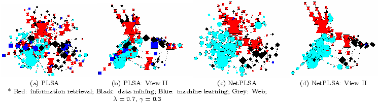
Specifically, we assign each author to one of the topics, by
![]() . We
then visualize the authors assigned to different topics with
different shapes and colors. The authors with the same shape thus
form a topical community summarized by the corresponding topic
model. As discussed in Section 2, the
authors in the same topical community are expected to be well
connected.
. We
then visualize the authors assigned to different topics with
different shapes and colors. The authors with the same shape thus
form a topical community summarized by the corresponding topic
model. As discussed in Section 2, the
authors in the same topical community are expected to be well
connected.
Figure 3 (a) and (b) present the topical communities extracted with the basic PLSA model, and Figure 3 (c) and (d) present the topical communities extracted with NetPLSA. With PLSA, although we can still see that lots of vertices in the same community are located closely, there aren't clear boundaries between communities. A considerable number of community members are scattered freely on the network (geometrically far from each other). On the other hand, when we regularize PLSA with the coauthor network, we see that the different communities can be identified clearly. Most authors assigned to the same topical community are well connected and closely located, which presents a much ``smoother'' pattern than Figure 3 (a) and (b).
Can we quantitatively prove that NetPLSA extracts better communities than PLSA? We have shown that network structure can help extracting topics. What about the reverse? Can a topic model of text help the network analysis?
| Methods | Cut Edge | R. Cut/ | Community
Size ( |
|||
| weights | N. Cut | C1* | C2 | C3 | C4 | |
| PLSA | 4831 | 2.14/1.25 | 2280 | 2178 | 2326 | 2257 |
| NetPLSA | 662 | 0.29/0.13 | 2636 | 1989 | 3069 | 1347 |
| NCut | 855 | 0.23/0.12 | 2699 | 6323 | 8 | 11 |
*Avg author weight: C1: 2.5; C2: 2.4; C3: 2.3; C4: 1.8; All: 2.2
In Table 3, we quantitatively compare the performance of PLSA, NetPLSA, and a pure graph-based community extraction algorithm. We present the total weight of edges across different communities in column 2, and number of authors in each community in the rightmost 4 columns. Intuitively, if the communities are coherent, there should be many inner edges within each community and few cut edges across different communities. Clearly, there is significantly fewer cross community edges, and more inner community conductorships in the communities extracted by NetPLSA than PLSA. This means that NetPLSA indeed extracts more coherence topical communities than PLSA. Interestingly, we see that although Topic 4 (Web) in Table 2 is a coherent topic (more than 1300 authors are assigned to that topic), we cannot see a comparable number of members of this topical community from Figure 3, where we removed low degree authors and singletons (especially from Figure 3 (c) and (d)). This is because unlike IR, data mining and machine learning, ``Web'' is more an application field to the researchers than a focused research community, where many authors are from external communities and applying their techniques to the Web domain, and publishing papers to WWW. People purely assigned to the ``WWW'' topic either didn't publish many papers, or are not well connected.
One may argue that in terms of inner/inter-community links
alone, a community discovery algorithm which purely relies on the
network structure may achieve a better performance. Indeed, what
if we use the graph-based regularizer alone (by setting the
![]() in Equation 3 and including some constraints)? A quick
answer maybe ``you can get intensively connected communities
but you may not get semantically coherent ones''. To verify
this, we compare our results with a pure graph-based clustering
method. Specifically, we compare with the Normalized Cut (NC)
clustering algorithm [24],
which is one of the standard spectral clustering algorithms. By
feeding the algorithm4 with the coauthor matrix, we also
extract four clusters (communities).
in Equation 3 and including some constraints)? A quick
answer maybe ``you can get intensively connected communities
but you may not get semantically coherent ones''. To verify
this, we compare our results with a pure graph-based clustering
method. Specifically, we compare with the Normalized Cut (NC)
clustering algorithm [24],
which is one of the standard spectral clustering algorithms. By
feeding the algorithm4 with the coauthor matrix, we also
extract four clusters (communities).
We present two other objectives of graph segmentation in the third column of Table 3, namely the ``normalized cut [24]'' and ``ratio cut [6]''. They respectively normalize the cross edges between two communities with the number of inner edges and the size of vertices in each community. If we solely consider the cut edges, it is hard to tell whether Normalized Cut or NetPLSA segments the network better, since one has a smaller ``minimum cut'' and the other has a smaller ``normalized cut''. However, in terms of topical communities, we see that our results are more reasonable. Community 3 and 4 of NC are extremely small. There is no way that they could represent a real research community, or any of the 4 conferences. Indeed, graph-based clustering algorithms are often trapped with small communities when the graph structure is highly skewed (or disconnected). In the network, we find that both cluster 3 and 4 are isolated components in the network (no out edges). They are both very coherent ``topological communities'', but not good topical communities, since the semantic information they represent is too narrow to cover a general topic. The involving of a topic model alleviates this sensitivity by bridging disconnected components with implicit topical correlations. This also guarantees semantical coherency within communities.
Even when a pure graph-based method extracts a perfect community, without the help of the topic model, it's hard to get a good topical summary of such a community. Community 1 of Normalized Cut well overlaps with the ``information retrieval'' community we got by NetPLSA. However, if we estimate a language model from the authors assigned to this community, we ends up with top probability words like ``web'', ``information'', ``retrieval'', ``neural'', ``learning'', ``search'', ``document'', etc (with MLE, and removing stop words). The semantics looks like a mixture and not as coherent as the NetPLSA results in Table 2. This is because in reality, an author usually works on more than one topics. Even when she is assigned to one community (even if assigned softly), we still need to exclude her work on other areas from the summary of this community, which cannot be achieved with just the network structure. This problem is naturally solved with the involvement of a topic model, which assumes that a document covers multiple topics, and treats different words in a document differently.
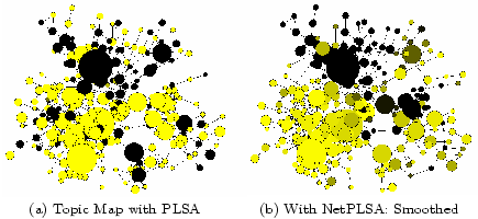
Another basic task of TMN is to generate a map on the network
for every topic. We use the probability ![]() as the weighting function
as the weighting function ![]() . We use the shades of a vertex to
visualize the probability
. We use the shades of a vertex to
visualize the probability ![]() , where a darker vertex has a larger
, where a darker vertex has a larger
![]() . As in Section
2, in a good topic map, the shades of
adjacent vertices should be smooth.
. As in Section
2, in a good topic map, the shades of
adjacent vertices should be smooth.
In Figure 4, we visualize the topic
map of ``information retrieval'' with the spring embedded view of
the 4-CONF network. The darker a vertex is, the more likely the
author belongs to the information retrieval community. From
Figure 4 (a), we see that although a
topic map could also be constructed with PLSA alone, the
distribution of the topic on the network is desultory. It is hard
to see where the topic origins, and how it is propagated on the
network. We also see that PLSA likes to make extreme decisions,
where an author is likely to be assigned an extremely large or
small ![]() . In Figure
4 (b), however, we see that through the
regularization with the coauthor network, the topic map is much
smoother. We can easily identify the densest region of the topic
``IR'', and see it gradually propagates to the farther areas.
Transitions between IR and non-IR communities are smooth, where
the color of nodes changes from the darkest to the lightest in a
gradational manner.
. In Figure
4 (b), however, we see that through the
regularization with the coauthor network, the topic map is much
smoother. We can easily identify the densest region of the topic
``IR'', and see it gradually propagates to the farther areas.
Transitions between IR and non-IR communities are smooth, where
the color of nodes changes from the darkest to the lightest in a
gradational manner.
As discussed in [19,20,9], the weblog/blog data is a new genre of text data which is associated with rich demographic information. It is thus a suitable test bed for text mining problems with spatial analysis. Following [19], we collect weblog articles about a focused topic, by submitting a focused query to Google Blog Search5, and crawling the content and geographic information of returned blog posts from their original websites. In this experiment, we use one of the data sets in [19], the Hurricane Katrina dataset. We also create a new dataset, with blog articles which contains the word ``weather'' in their titles. The basic statistics of the datasets are shown in Table 4.
| Dataset | Time Span | Query | |
| Katrina | 4341* | 8/16/05 - 10/04/05 | ``hurricane katrina'' |
| Weather | 493 | 10/01/06 - 9/30/07 | ``weather'' in Title |
For both datasets, we create a vertex for every state in the U.S. and an edge between two adjacent states.
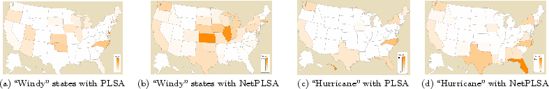
We use the model in Section 4.2 to extract topics with the context of geographic network structure. We then use the Many Eye visualization service6 to visualize the spatial topic distribution of the one subtopic in hurricane Katrina. The subtopic discusses about the storms in Katrina, and in its successor hurricane Rita. Comparing Figure 5 (a) with Figure 5 (b), we see that the geographic distribution of topic is not dramatically different. This is reasonable, since the topic plotted in both figures is the same topic. However, we can still feel the difference between the figures: the topic distribution of Figure 5 (b) is much smoother than that in Figure 5 (a). Assume that a user does not know about hurricane Katrina or hurricane Rita, it is hard for her to guess where the events occurred from Figure 5 (a). People in Maine, Michigan, and Rhode Island seem to particularly focus on this topic, even more than people in Florida, Louisiana, and Mississippi (because of the sparsity of data in those states). From Figure 5 (b), however, we clearly see that the topic is densest along the Golf of Mexico, and gradually dilutes when it goes north and west. It is also clear that the discussion on this topic is denser in the west US than in the east. This is consistent with the reality, where the topic origins in the southeast coast, and gradually propagates to other states. In Figure 5 (b), we also see that the topic propagates smoothly between adjacent states. This also shows that our model could alleviate the overfitting problem of PLSA.
Let us show the results with another dataset, the Weather
dataset in Table 4. Intuitively, when a
user was discussing about weather in her blogs, the topics she
chose to write about would be affected by where she lived. Since
the topic ``weather'' is very broad, we guide the mixture model
with some prior knowledge, so that it could extract several
topics which we expect to see. Following [18], this is done by changing
the MLE estimation of ![]() in M step (Equation 11) into a
maximum a posterior (MAP) estimation. We extract 7 topics from
the Weather dataset. We use ``wind'' and ``hurricane'' as the
prior for two of the topics, so that one of the output topic will
be about the windy weather, and another will be about hurricanes.
Table 5 compares the prior-guided
topic models extracted from the Weather dataset. We see that with
the network based regularizer, we indeed extract more coherent
topics.
in M step (Equation 11) into a
maximum a posterior (MAP) estimation. We extract 7 topics from
the Weather dataset. We use ``wind'' and ``hurricane'' as the
prior for two of the topics, so that one of the output topic will
be about the windy weather, and another will be about hurricanes.
Table 5 compares the prior-guided
topic models extracted from the Weather dataset. We see that with
the network based regularizer, we indeed extract more coherent
topics.
| PLSA | NetPLSA | ||
| ``wind'' | ``hurricane'' | ``wind'' | ``hurricane'' |
| windy | dean | windy | hurricanes |
| severe | storm | f | storms |
| pm | mexico | hi | tropical |
| thunderstorm | texas | cloudy | atlantic |
| hail | category | lo | season |
| watch | jamaica | lows | erin |
| blah | oil | highs | houston |
| probability | tourists | mph | louisiana |
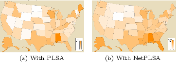
In Figure 6, we visualize the
geographic distributions of two weather topics over the US
states. Comparing to the distributions computed with PLSA, we see
that with NetPLSA, we can get much smoother distributions. PLSA
assigns extremely large (close to 1) ![]() of the topic ``windy'' to Delaware, and
``hurricane'' to Hawaii. On the other hand, it assigns
surprisingly low probability of ``windy'' to Texas. It also
assigns extremely low probability of ``hurricane'' to
Mississippi, Alabama and Georgia, although they are among the
most vulnerable states to hurricanes. Through the regularization
with states network, we see that this problem is alleviated.
Northern midwest states and Texas are identified as windy states,
especially Illinois (where the ``windy city'' Chicago locates).
The southeast coasts, especially the states alone the Golf of
Mexico (Florida as a representative), are identified as
``hurricane'' states.
of the topic ``windy'' to Delaware, and
``hurricane'' to Hawaii. On the other hand, it assigns
surprisingly low probability of ``windy'' to Texas. It also
assigns extremely low probability of ``hurricane'' to
Mississippi, Alabama and Georgia, although they are among the
most vulnerable states to hurricanes. Through the regularization
with states network, we see that this problem is alleviated.
Northern midwest states and Texas are identified as windy states,
especially Illinois (where the ``windy city'' Chicago locates).
The southeast coasts, especially the states alone the Golf of
Mexico (Florida as a representative), are identified as
``hurricane'' states.
In this section, we showed that with network based regularization, the NetPLSA model outperforms PLSA. It also extracts more robust topical communities than solely graph-based methods. NetPLSA generates coherent topics, topologically and semantically coherent communities, smoothed topic maps, and meaningful geographic topic distributions.
Statistical topic modeling and social network analysis have little overlap in existing literature. Statistical topic modeling [10,4,28,26,19,20,15] uses a multinomial word distribution to represent a topic, and explains the generation of the text collection with a mixture of such topics. However, none of these existing models considers the natural network structure in the data. In the basic models such as PLSA [10] and LDA [4], there is no constraint other than ``sum-to-one'' on the topic-document distributions. [25] uses a regularizer based on KL divergence, by discouraging the topic distribution of a document from deviating the average topic distribution in the collection. We propose a different method, by regularizing a statistical topic model (e.g., PLSA) with the network structure associated with the data.
Contextual text mining [28,26,19,20] is concerned with modeling topics and discovering other textual patterns with the consideration of contextual information, such as time, geographic location, and authorship. Our work is the first attempt where a network structure is considered as the context in topic models.
Social network analysis has been a hot topic for quite a few years. Many techniques have been proposed to discover communities [11,1], model the evolution of the graph [13], and understand the diffusion of social networks [9,14]. However, the rich textual information associated with the social network is ignored in most cases.
Although there has been some existing explorations [7,17,16,2], there has not been a unified way to combine textual contents with social networks. Indeed, [31] proposes a probabilistic model to extract e-communities based on the content of communication documents, but they leave aside the network structure in their model. Cohn and Hofmann proposed a model which combines PLSA and PHITS on the web graph [7]. Both topic and link are modeled as generated from a probabilistic mixture model. Their model, however, assumes a directed graph and does not directly optimize the smoothness of topics on the graph. To the best of our knowledge, combining topic modeling with graph-based harmonic regularization is a novel approach.
The graph-based regularizer is related to existing work in machine learning, especially graph-based semi-supervised learning [33,29,3,32] and spectral clustering [6,24]. The optimization framework we propose is closely related to [34], which is probably the first work combining a generative model with graph-based regularizer. Our work is different from theirs, as their task is semi-supervised classification, while we focus on unsupervised text mining problems such as topic modeling. NetSTM is a generalization of harmonic mixture to multiple topics and unsupervised learning.
The concrete applications we introduced in Section 4 are also related to existing work on author-topic analysis [26,20], spatiotemporal text mining [19,20], and blog mining [9,19]. [30] explores co-author network to estimate the Markov transition probabilities between topics, which uses the network structure as a post processing step of topic modeling. Our work leverages the generative topic modeling and discriminative regularization in a unified framework.
In many knowledge discovery tasks, we encounter a data collection with both abundant textual information and a network structure. Statistical topic models extract coherent topics from the text, while usually ignoring the network structure. Social network analysis on the other hand, tends to focus on the topological network structure, while leaving aside the textual information. In this work, we formally define the major tasks of topic modeling with network structure. We propose a general solution of text mining with network structure, which optimizes the likelihood of topic generation and the topic smoothness on the graph in a unified way. Specifically, we propose a regularization framework for statistical topic models, with a harmonic regularizer based on the network structure. The general framework allows arbitrary choices of the topic model and the graph based regularizer. We show that with concrete choices, the model can be applied to tackle real world text mining problems such as author-topic analysis, topical community discovery, and spatial topic analysis.
Empirical experiments on two different genres of data show that our proposed method is effective to extract topics, discover topical communities, build topic maps, and model geographic topic distributions. It improves both pure topic modeling, and pure graph-based method.
There are many potential future directions of this work. It is interesting to see how other topic models and regularizers can be adopted (e.g., LDA, normalized cut, etc). It is also interesting to study how the special properties of social networks can be considered in this framework, such as the small world property. Utilizing such a model to model the evolution of topics and community is also a promising direction, which requires the modeling of time dimension.

![\begin{displaymath} X^{(t+1)} = X^{(t)} - \gamma[HQ(X^{(t)};\Psi_n)]^{-1}\bigtriangledown Q(X^{(t)};\Psi_n) \end{displaymath}](fp806-mei-img113.png)