Enhanced Hierarchical Classification via Isotonic Smoothing

Kunal Punera

Yahoo! Research

701 First Ave.

Joydeep Ghosh

University of Texas at Austin

Austin, TX 78712

Abstract:

Hierarchical topic taxonomies have proliferated on the World Wide Web [5,18], and exploiting the output space decompositions they induce in automated classification systems is an active area of research. In many domains, classifiers learned on a hierarchy of classes have been shown to outperform those learned on a flat set of classes. In this paper we argue that the hierarchical arrangement of classes leads to intuitive relationships between the corresponding classifiers' output scores, and that enforcing these relationships as a post-processing step after classification can improve its accuracy. We formulate the task of smoothing classifier outputs as a regularized isotonic tree regression problem, and present a dynamic programming based method that solves it optimally. This new problem generalizes the classic isotonic tree regression problem, and both, the new formulation and algorithm, might be of independent interest. In our empirical analysis of two real-world text classification scenarios, we show that our approach to smoothing classifier outputs results in improved classification accuracy.

H.4.mInformation SystemsInformation Storage and Retrieval Algorithms, Experimentation Hierarchical Classification, Taxonomy, Regualrized Isotonic Regression, Dynamic Programming

1 Introduction

Hierarchical taxonomies play a crucial role in the organization of knowledge in many domains. Taxonomies structured as hierarchies make it easier to navigate and access data as well as to maintain and enrich it. This is especially true in the context of a vast dynamic environment like the World Wide Web where the amount of available information is overwhelming; this has lead to a proliferation of human constructed topic directories [5,18] Because of their ubiquitousness there has been considerable interest in automated methods for classification into hierarchical taxonomies, and numerous techniques have been proposed [6,14,3,10]. In this paper, we will introduce ideas as well as algorithms that serve to further improve the accuracy of hierarchical classification systems.

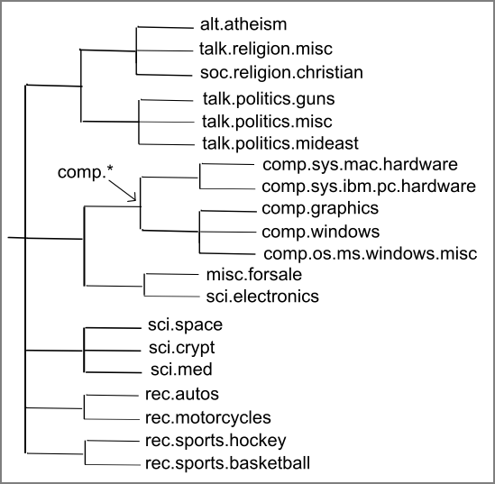
While studying systems that classify instances into a taxonomy of classes we have to consider many different aspects of the problem. Some of these result from variations in characteristics of taxonomies themselves, such as whether or not instances are allowed to belong to classes at the internal nodes, while others are because of variations in the way classifiers are trained. We illustrate some of these issues by considering a few real-world scenarios. We will refer to these scenarios throughout the paper to place the applicability of our approaches in context. A taxonomy constructed on the 20-newsgroups dataset (Figure 1) will be used as a running example below.

• Scenario I: In the 20-newsgroups dataset all instances belong to leaf-level classes of the taxonomy (Figure 1). Suppose while learning the classifiers at each node, the positive (negative) set of instances are from leaf nodes within (outside) the subtree rooted at the node. For instance, for the classifier at the node comp.*, the positive document set comes from all computer related leaf-level classes, and the negative document set from all other classes. In this scenario, when a test document is classified as belonging to a class (say, comp.graphics) all internal classes on the path to the root must also be labeled positive. Similarly, if an internal node class is labeled as positive for a document at least one of the leaf-level classes under it must also be labeled positive.

• Scenario II: There exist taxonomies in which instances sometimes belong to classes that are internal nodes and not to any leaf-level classes. Once again consider the taxonomy for the 20-newsgroups dataset. We can imagine that the internal node comp.* might contain documents that discuss computers in general, and not software or hardware (MS or Mac) in particular. Now, if the classifiers are learned as in Scenario I - distinguishing the documents within the subtree from those outside - we can see that, if a node is labeled positive for a document then all internal classes on the path to the root must also be labeled positive. However, since there is no restriction that the document be associated to any leaf-level classes, it is not necessary that at least one child of the node also be labeled positive.

Figure 1: Taxonomy of classes in the 20-newsgroups dataset.

In addition to these two scenarios several other variations in the structure of the taxonomy and construction of classification problems can be imagined. A common aspect, however, is the mechanism for classifying new data instances into the taxonomy. For this purpose each learned classifier is applied to the new data instance to obtain membership scores. The membership scores outputted may be binary, or they can be thresholded to determine the classes that are labeled positive.

However, from our discussion of different classification scenarios we know that in many cases these membership scores are related across nodes. For example, in case of the 20-newsgroups dataset under Scenario I, it cannot be that the class comp.graphics is labeled positive and class comp.* is labeled negative for the same document. In other words, due to characteristics of taxonomies and specifics of classifier training, relationships between classes in a taxonomy lead to relationships between outputs of their classifiers. Furthermore, these properties can also be devised from knowledge of the application domain or the behavior of classification algorithms.

OUR CONTRIBUTION.

The central idea in this paper is that once we have identified the exact property that the outputs of classifiers in a taxonomy must satisfy, we can post-process the classification scores to enforce these constraints. Whenever classifier scores violate these constraints we will replace them with consistent scores that are as close as possible to the original ones. Since only a few classifiers are likely to make mistakes on any one instance it is hoped that the outputs of the incorrect ones will be modified appropriately.

In this paper, we will formulate the problem of enforcing constraints on classifier outputs under Scenarios I and II as regularized tree isotonic median regression problems. These are generalizations of the classic isotonic regression problem. We will also provide a dynamic programming based algorithm that finds the optimal solutions to these more general optimization problems in $O(n^2\log{n})$ time; this is equal to the best known algorithms for the classic problem. This new problem formulation and algorithm might be of interest independent of the hierarchical classification task. We will present empirical analysis on a real-world text dataset to show that post-processing of classifier scores results in improved classification accuracy.

2 Regularized Isotonic Regression

In this section we will formulate the problem of smoothing classifier outputs as a regularized isotonic regression problem and give an efficient algorithm to solve it optimally. Before we proceed, however, let us establish some notation.

NOTATION.

Let ${\cal C}$ be a set of $n$ classes in a taxonomy that have a one to one mapping with the nodes of a rooted tree $T$. Let $\mathrm{leaf}(T)$ and $\mathrm{root}(T)$ represent the set of leaves and the root of the tree $T$ respectively. Let $v$ be a node of $T$ (written as $v \in T$) and let $T_v$ denote the subtree rooted at $v$. We will refer to a node in the tree $T$ sometimes as a class. We use $\mathrm{parent}(v)$ to denote the parent of $v$ in $T$, $\mathrm{child}(v)$ to denote the set of all immediate children of $v$ in $T$. Let $\cal D$ denote the set of all data instances. These instances belong to one of the classes in $\cal C$; this mapping is denoted by function $\tau$. Depending on the real-world scenario being modeled, $\tau$ may map instances to only a subset of classes in $\cal C$.

Each class $v \in T$ has associated with it a function $c_v:{\cal D} \rightarrow [0,1]$, where $c_v(d)$ is the degree of membership of instance $d$ in class $v$. In our application setting this value can be interpreted as a posterior probability; using an appropriate threshold it can be rounded to a boolean value. An instance $d$ can be represented by a function $x_d$ where the $x_d(v)$ represents the value $c_v(d)$. Since each class corresponds to a unique node in the taxonomy $T$, we can think of $x(.)$ as being values assigned to nodes of $T$. Henceforth we will use $T$, $v$, and $x(v)$ as metaphors for the taxonomy, a class or a node, and the classifier score or node value respectively. In our application settings we distinguish between an instance belonging to a class (implying that $\tau(d)=v$) and associating with a class (implying that because of the way classifiers were trained we expect $x_d(v)=1$). However, when it is clear from context, we will use the term belonging to refer to both situations.

1 Formulation

Consider the Scenario I described above. The data instances under this setting always belong to one of the leaf-level classes¹; the range of $\tau$ is $\mathrm{leaf}(T)$. Moreover, for an internal node $v \in T$ the positive set of instances for training classifier $c_v$ is the union of instances that belong to $\mathrm{leaf}(T_v)$. Consequently, this means that the true labeling of any instance is a leaf-level class $v$ and all its parents on the path to the $\mathrm{root}(T)$. This property can be succinctly stated as follows:

Property 2.1 (Strict Classification Monotonicity)  
An instance belongs to a class in the taxonomy if and only if it belongs to at least one of its children classes.

This means that we expect $x(v)=1 \iff \exists u \in \mathrm{child}(v): x(u)=1$.

However, as each classifier $c_v$ processes the instances independently of other classifiers, they miss this intuitive relationship amongst classifier outputs; $x(\cdot)$ need not satisfy Property 2.1. Hence, we need to transform $x(\cdot)$ into smoothed classifier scores $y(\cdot )$ such that elements in $y(\cdot )$ satisfy the monotonicity property.

We have defined the monotonicity property for boolean classification values, so we first consider a natural generalization in order to handle real-valued classifier scores. Suppose $y(\cdot )$ are the smoothed classifier scores, then they satisfy generalized strict classification monotonicity property if for every internal node $v$, with children $u_1, \ldots, u_\ell$, $y(v) = max\{y(u_1),\ldots,y(u_{\ell})\}$, i.e., the smoothed score of an internal node is the equal to the maximum of its children's smoothed scores. Note that generalized monotonicity ensures that whenever an instance is associated with a class $v$, first, it's also associated with $\mathrm{parent}(v)$, and second, it's also associated with at least one child of $v$, if any.

Moreover, we assume that the individual classifiers have reasonable accuracy and so we want to obtain $y(\cdot )$ that is as close as possible to the original scores $x(\cdot)$ while satisfying the monotonicity property. This gives us the following problem:

Problem 2.2   Given classifier scores $x(\cdot)$, find smoothed scores $y(\cdot )$ that minimize

$$\sum_{v \in T}\vert x(v) - y(v) \vert$$ (1)

while satisfying the generalized version of Property 2.1.

Here we compute the distance between $x(\cdot)$ and $y(\cdot )$ via the $L_1$ distance, however, any other distance measure could also have been used. We chose $L_1$ distance over $L_2$ because of its robustness to noise.

Figure 2: Examples of hierarchies with scores on nodes. The green circles highlight correct scores and the red squares erroneous ones.

Now consider Scenario II mentioned above. In this situation there exist some instances that belong only to internal nodes, and not to any of the leaf nodes. Moreover, the positive set of instances used for training classifier $c_v$ for node $v \in T$ is the union of instances that belong to all nodes in the subtree $T_v$. This implies that the true labels for an instance will be a node $v \in T$ and all its parents on the path to $\mathrm{root}(T)$. However, unlike Scenario I, its no longer necessary for at least one child of $v$ to also be included in the true labels.

As is evident, this relationship between classifiers scores is not covered by Property 2.1, which enforces that every instance must belong to at least one leaf node. In order to incorporate situations such as Scenario II we state the relaxed monotonicity property.

Property 2.3 (Relaxed Classification Monotonicity)   The classifier score of a node is always greater than or equal to the classifier scores of its children.

Let $y(\cdot )$ be the smoothed classifier scores, then $y(\cdot )$ satisfies relaxed monotonicity if for every internal node $v$, with children
$u_1, \ldots, u_\ell$, $y(i) \geq max\{y(u_1),\ldots,y(u_{\ell})\}$. Finding such a $y(\cdot )$ while minimizing Equation (1) will help us correct some of the errors introduced by the classifiers.

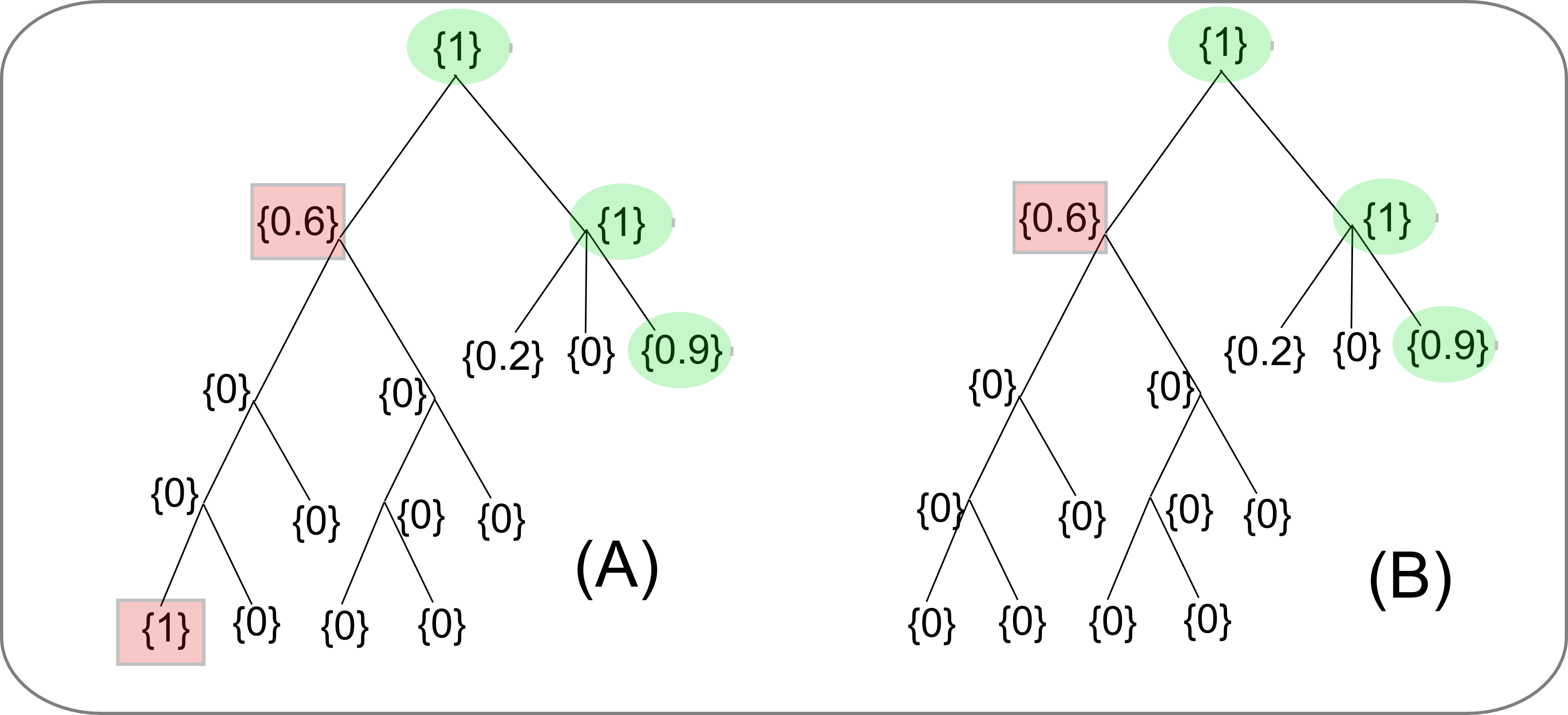
For instance, consider the classification scores on the tree A in Figure 2. The nodes that are shaded by a red square represent the errors in the classification. The leaf-node with score 1 clearly violates monotonicity constraints since its ancestors' scores are lower than its own. This error will be corrected since it is more expensive to increase all the ancestors' scores than it is to reduce the erroneous node's score.

However, the relaxed monotonicity property will allow certain other types of errors that might occur frequently. For example, consider the error node in tree B of Figure 2. This node doesn't violate the relaxed monotonicity property since its parent's score is higher than its own. However, this error node's score would have been corrected by the strict monotonicity property, which would have required at least one child of the error node to have the same score. It would have cost less (in terms of Equation (1)) to reduce 0.6 to 0, than to increase a whole series of values from 0 to 0.6.

In order to correct the latter type of errors we introduce an additional regularization term in our objective function, which penalizes violations of strict monotonicity. Hence, while we will accept smoothed scores $y(\cdot )$ that satisfy the relaxed monotonicity property as valid solutions, they will be charged for all the violations of the strict monotonicity constraints. In the case of the tree B in Figure 2, if the penalty is high enough, it will cost lesser to reduce the error node's value to 0 than to leave the scores as it is, thus correcting the false positive error. Regularization can also be useful for reducing false negative errors when it is cheaper to increase a child node value than to pay the penalty.

Taking into account this regularization we state a new problem:

Problem 2.4 (Regularized Tree Isotonic Regression)   Given classifier scores $x(\cdot)$, find smoothed scores $y(\cdot )$ that minimize

$$% latex2html id marker 226 \sum_{v \in T} w_v\cdot\vert x(... ...}}\gamma_v\cdot \left(y(v) - \mathrm{max}\{y(u_i)\}\right)$$ (2)

while satisfying Property 2.3, where $w_v$ and $\gamma _v$ are node-specific weights and penalties, respectively.

In Equation (2) $w_v$ are the node-specific weights that control the amount each classifier's score contributes to the total cost. We can set these weights to reflect our belief in the classifier's accuracy. The $\gamma _v$ values are weights that control the extent to which violations of strict monotonicity constraints are prohibited. These penalty values can also be set in a node-specific fashion.

Problem 2.4 is a regularized version of isotonic regression problem on trees which has been widely studied [1,13]. It reduces to the standard isotonic regression when all the penalties are set to 0. Moreover, we can also enforce strict monotonicity (Property 2.1) by setting $\gamma_v=\infty$.

Figure 3: Algorithm to solve Problem 2.2. Array $x$ contains the original classifier scores and $\hat{x}$ is the set of unique values in $x$. $w_v$ denote the node-specific weights. BUILDERRORSTRICT constructs functions $\mathrm{err}(\cdot,\cdot)$ and $\mathrm{val}(\cdot,\cdot)$ which are then used by ISOTONESMOOTH to find the smoothed scores $y(\cdot )$.

2 Algorithm for the case $\mathbf{\gamma=\infty}$

We first present an algorithm for the special case of penalty $\gamma=\infty$; in fact, we'll solve Problem 2.2. The dynamic programming based algorithm presented in this section is similar in structure to the more general algorithm presented in the next section, and serves as a good starting point in introducing the ideas behind the approach.

Before we describe the algorithm we will discuss a crucial detail of the structure of the problem. We show that the optimal smoothed scores in $y(\cdot )$ can only come from the classifier scores $x(\cdot)$.

Lemma 2.5   For Problem 2.2 there exists an optimal solution, $y(\cdot )$, where, for all $i \in T$ there is a $j \in T$ such that $y(i) = x(j)$.

Consider the maximal connected subtree $T'$ of nodes in $T$ such that (1) $i \in T'$, and (2) for all $j \in T'$, $y(j) = y(i)$. If $y(i)$ is not the median of the set of scores $\{x(j) \mid j \in T' \}$, then we can push $y(i)$ closer to the median by a small amount and decrease the cost of the solution given by Equation (1); this follows since the median is the minimizer for $L_1$ distance.

This result shows that in the optimal solution the smoothed score for each node will come from a finite set of values. Note that this result also holds for the case of weighted $L_1$ distance. In this case each weighted node in the tree can be considered as multiple nodes, which number proportional to the weight, and which always have the same score. In this case too, the minimizer remains the median of this expanded graph. And hence the smoothed score values come from the finite set of original values.

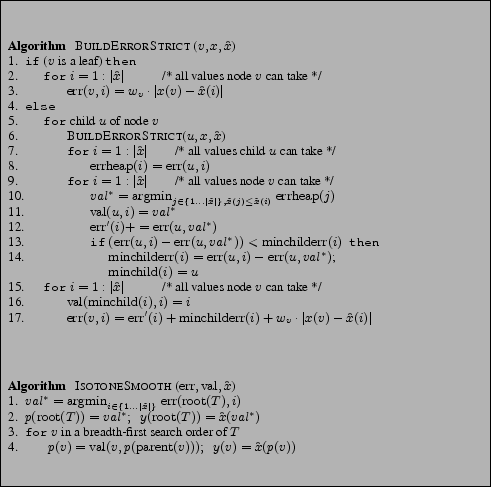
To solve Problem 2.2 optimally we construct a dynamic programming based method (pseudo-code in Figure 3). The program consists of two main algorithms, (1) BUILDERRORSTRICT, which builds up the index function $\mathrm{val}$ and error function $\mathrm{err}$, and (2) ISOTONESMOOTH, which uses the $\mathrm{val}$ function to compute the optimal values for each node in the tree. Let $\hat{x}$ be the set of unique values in $x(\cdot)$, and let $i$ be an index into this set. Then index function $val(v,i)$ holds the index of the value that node $v$ should take in the optimal solution when its parent takes the value $\hat{x}(i)$. In other words, when $y(\mathrm{parent}(v))=\hat{x}(i)$ then $y(v)=\hat{x}(\mathrm{val}(v,i))$. In order to compute the function $\mathrm{val}$, BUILDERRORSTRICT computes for each node $v$ the function $\mathrm{err}(v,i)$, which holds the total cost of the optimal smoothed scores in the subtree $T_v$ when $y(v)=\hat{x}(i)$.

Initially BUILDERRORSTRICT is invoked with $\mathrm{root}(T)$ as a parameter. The function then recursively calls itself (step 6) on the nodes of $T$ in a depth-first order. While processing a node $v$, for each possible value $\hat{x}(i)$ that $v$ can set itself to, BUILDERRORSTRICT finds the best values for its children that are less than or equal to $\hat{x}(i)$ (step 10). All children of $v$ are assumed to be set to their best possible values (step 11) and their costs (errors) are added up (step 12). Also, since in the final solution one of the children's value has to be equal to value of $v$, BUILDERRORSTRICT maintains information about the child that would cost the least (steps 13 & 14) to move to $\hat{x}(i)$ (step 16). At the end the cost of all children and the additional cost of the ``minchild'' that is moved are added (step 17) to obtain the cost for the current node.

To demonstrate the correctness of this algorithm, we show that the restriction of the optimal solution to a subtree is also the optimal solution for the subtree under the monotonicity constraint imposed by its parent.

Consider the subtree rooted at any non-root node $v \in T$. Now suppose the smoothed score $y(\mathrm{parent}(v))$ is specified. Then, let $z(\cdot)$ be the smoothed scores of the optimal solution to the regularized tree isotonic regression problem for this subtree, under the additional constraint that $z(v) \leq y(\mathrm{parent}(v))$. Note that if $v$ is chosen as ``minchild'' in algorithm BUILDERRORSTRICT above, the constraint is $z(v)=y(\mathrm{parent}(v))$.

Lemma 2.6   For all nodes $i$ in the subtree of $v$, $y(i) = z(i)$.

Consider a smoothed solution $w(\cdot)$ where $w(i) = z(i)$ for all nodes $i$ in the subtree of $v$, and $w(i)=y(i)$ otherwise. It is clear that since $z(\cdot)$ obeys the monotonicity property and
$z(v) \leq y(\mathrm{parent}(v))$, the solution $w(\cdot)$ obeys the monotonicity property. Now, the cost $c(w)$ is the sum of the cost for the smoothed scores $z(i)$ in the subtree of $v$ and the cost for the scores $y(k)$ for all other nodes. Thus, the difference between $c(w)$ and $c(y)$ is just the difference in costs for $z(i)$ and $y(i)$ in the subtree of $v$, for which we know that $z(\cdot)$ is the optimal. The lemma follows.

Theorem 2.7   Algorithm ISOTONESMOOTH in Figure 3 solves Problem 2.2 exactly.

The algorithm computes up the optimal smoothed scores for each subtree, i.e., the $\mathrm{err}(\cdot,\cdot)$ arrays, while maintaining Property 2.3 for every possible smoothed score of the parent. Further, the child that costs the least to move from its optimal position to the parent value is moved. This causes the least increase in the cost in Equation (1). Hence, the solution computed for each possible smoothed value of the parent is optimal. By Lemma 2.5, the parent can take only finitely many smoothed scores in the optimal solution, and by Lemma 2.6, combining the optimal smoothed scores for subtrees yields the optimal smoothed scores for the entire tree.

COMPLEXITY. Let $\vert T\vert = n$, and so $\vert\hat{x}\vert$ can at most be $n$. The dynamic programming table takes $O(n)$ space per node, and so the total space required is $O(n^2)$. Next, we consider the running time of the algorithm. In the algorithm BUILDERRORSTRICT-I, step 2 takes $O(n^2)$ time, step 7 takes $O(n^2)$ time amortized over all calls (this loop is called for each node only once), and the loop in step 9 can be done in $O(n^2\log{n})$ time by storing $\mathrm{errheap}$ values in a heap and then running over the values $i \in \{1\ldots\vert\hat{x}\vert\}$ in descending order of $\hat{x}(i)$. Hence, the total running time is $O(n^2\log{n})$. Note that this is same as the best time complexity of previously known algorithms for the non-regularized forms of tree isotonic regression [1].

3 Algorithm for Regularized Tree Isotonic Regression

In the previous section we presented an algorithm to solve Problem 2.2. In this section we give an algorithm that solves the more general regularized isotonic regression problem exactly. The main difference between the two problems is that in the latter case the hard constraint of a parent's value being equal to at least one of its children's value is enforced via soft penalties. These violations of the strict monotonicity rule are charged for in the objective function, so that if the cost of incurring the penalties is lower than the improvement in $L_1$ error, the optimal solution will contain violations. This makes the current problem much tougher to solve. When constraints were strict each child only had two ways it could set its own value: equal to the best possible value less than the parent's value or equal to the parent's value. In the current problem because penalties are soft, the child has more options of values it can set itself to. However, we show that this set of possible values is still finite.

Here we prove that the central result (Lemma 2.5) which facilitated the algorithm in Figure 3 also holds for the modified objective function Equation (2).

PRELIMINARY FACTS.

Consider the maximal connected subtree $T'$ of nodes in $T$ such that (1) $i \in T'$, and (2) for all $j \in T'$, $y(j) = y(i)$. Let $m$ be the median of the set of original scores $S_{T'}=\{x(j) \mid j \in T'\}$. The cost incurred by $T'$ through the first term of Equation (2) ($L_1$ distance between $x$ and $y$) is minimized when $y(i)= m$. As we raise or lower $y(i)$ the increase in this cost is piecewise-linear, with the discontinuities at the values in the set $S_{T'}$. In other words, in between any two adjacent values in $S_{T'}$ the rate of change in the $L_1$ cost is constant (we denote this rate by a function $r_m(\cdot)$).

Now lets consider the cost due to penalties. Let $u$ be the ``maximal'' node in $T'$, such that $\mathrm{parent}(u) \ni T'$. Note that, as $T'$ is connected and is a tree, there is a unique such node. Also, let $\{v_i\}\in T'$ be a set of nodes such that at least one child of each $v_i$ is not in $T'$. Some elements in the set $P_{T'}=\{\mathrm{parent}(u),\mathrm{child}(\{v_i\})\}$ are involved in penalties for having values different from $y(i)$. This cost from penalties also changes in a piecewise-linear fashion with possible discontinuities at the values in the set $P_{T'}$. Let us denote the rate of change of penalty-based cost as $r_p(\cdot)$.

Lemma 2.8   For Problem 2.4 there exists an optimal solution, $y(\cdot )$, where, for all $i \in T$ there is a $j \in T$ such that $y(i) = x(j)$.

Let the cost of the optimal solution $y(\cdot )$ be $c(y)$. We will prove the above lemma for a solution $y(\cdot )$ that has the fewest distinct score values of all solutions that have cost $c(y)$. If this is not the case, then we'll show how $y(\cdot )$ can be converted to $y'(\cdot)$ that has fewer distinct score values.

Consider the maximal connected subtree $T'$ of nodes in $T$ such that (1) $i \in T'$, (2) for all $j \in T'$, $y(j) = y(i)$, and (3) there does not exist any $j \in T$ such that $y(i) = x(j)$. As mentioned above, since $y(i) \neq m$ (median of $S_{T'}=\{x(j) \mid j \in T'\}$), we can decrease the cost due to $L_1$ error at the rate of $r_m(y(i))$ by moving $y(i)$ towards $m$. Also, the cost due to penalties changes at the rate of $r_p(y(i))$ when we move $y(i)$. If the values $r_m(y(i)) \neq -r_p(y(i))$ then we can move $y(i)$ very slightly to decrease the overall cost.

Hence, we consider the case where $r_m(y(i)) = - r_p(y(i))$. Let $m_1 \in S_{T'}$ be the closest value to $y(i)$ in between it and $m$. Since the two rates of cost change counterbalance each other, small changes in $y(i)$ result in solutions with the exact same cost. In fact, we can move $y(i)$ to $m_1$ without any change in the overall cost, hence producing an optimal solution with satisfies the lemma. To see why this happens, consider that as we move $y(i)$ to $m_1$, $r_m(y(i))$ will not change as explained above. The quantity $r_p(y(i))$ will change if we encounter an element from the set $P_{T'}$ in between $y(i)$ and $m_1$. But this means that we can obtain a solution with cost $c(y)$ that has fewer distinct values, which violates our assumption. Another way in which $r_p(y(i))$ can change is if the maximal node $u$ stops/starts having the highest value of all its siblings (stops/starts getting penalized) as we move $y(i)$. However, it can be easily verified that this can only reduce the cost of the new solution further.

Figure 4: Algorithm to solve Problem 2.4. Array $x$ contains the original classifier scores and $\hat{x}$ is the set of unique values in $x$. $w_v$ and $\gamma _v$ denote the node-specific weights and penalties. BUILDERRORRELAX constructs functions $\mathrm{err}(\cdot,\cdot)$ and $\mathrm{val}(\cdot,\cdot)$ which are then used by ISOTONESMOOTH to find the smoothed scores $y(\cdot )$.

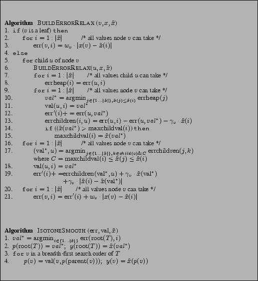Now we are ready to present the dynamic program to solve Problem 2.4 (pseudo-code in Figure 4). The input to the system is $x(\cdot)$, the original classifier scores; $\hat{x}$ is the set of unique values in $x$. The algorithm BUILDERRORRELAX, invoked on the root node, recurses over nodes of $T$ in a depth first order (step 6) and fills up the index function $\mathrm{val}$ and error function $\mathrm{err}$. The index function $\mathrm{val}(v,i)$ holds the index of the value that node $v$ should take in the optimal solution when its parent takes the value $\hat{x}(i)$, while the function $\mathrm{err}(v,i)$ stores the total cost of the optimal smoothed scores in the subtree rooted at $v$ when $y(v)=\hat{x}(i)$. In these respects, BUILDERRORRELAX is identical to the algorithm for the strict monotonicity property presented in Section 2.2. The main difference is that now the cost of the solution doesn't just come from the $L_1$ error, but also from the penalties. Hence, while picking a value for a child node we have to consider both the cost of the optimal solution in the subtree of the child and the cost of the child's value differing from the parent value. To add to the complexity, we have to consider the latter cost only when the child has the maximum value amongst its siblings.

While operating on a node $v$, for each possible value $\hat{x}(i)$ that $v$ can set itself to, BUILDERRORRELAX first obtains the best value assignments for its children that are less than or equal to $\hat{x}(i)$ (step 10). At this stage, only the cost of the optimal solutions in the subtree of a child is considered while determining its best value (step 8); for now the cost, due to penalties, of a child's value differing from $\hat{x}(i)$ is ignored. The $\mathrm{val}$ array entries of the children are set to these best values (step 11) and the costs are added up (step 12). While processing each child this way another table $\mathrm{errchildren}$ is populated with the additional cost of moving one of the children to be the maximum child under $v$ (step 13). Once all children values have been set this way, in a second pass the $\mathrm{errchildren}$ table is used to determine which child should be moved, and what value it should be moved to, so that the sum of the cost from its subtree and penalty w.r.t. the parent value is minimum (step 17). Once the child and its new value are determined, step 18 and step 19 update the $\mathrm{val}$ array and the cost of the current node $v$ respectively. Note that the initial assignment of values to children might not change in this second pass if the original child with the maximum value also costs the least once we take into account penalties. Once BUILDERRORRELAX has filled the $\mathrm{val}$ array, the function ISOTONESMOOTH uses it to compute the optimal values for each node in the tree.

To demonstrate the correctness of this algorithm, we first show that the restriction of the optimal solution to a subtree is also the optimal solution for the subtree under the constraints imposed by its parent. Consider the subtree rooted at any non-root node $v \in T$. Now suppose the smoothed score $y(\mathrm{parent}(v))$ is specified and also whether $v$ has the maximum value of its siblings in the optimal solution. If $v$ does not have the maximum value then let $z(\cdot)$ be the smoothed scores of the optimal solution to the regularized tree isotonic regression problem for this subtree, under the additional constraint that $z(v) \leq y(\mathrm{parent}(v))$. If $v$ does have the maximum value then let $z(\cdot)$ represent the optimal smoothed scores in $T_v$ such that they minimize $c(z) + \gamma_v \cdot \vert y(\mathrm{parent}(v))-z(v)\vert$ subject to $z(v) \leq y(\mathrm{parent}(v))$, where $c(z)$ is the cost of the subtree $T_v$ under $z(\cdot)$.

Lemma 2.9   For all nodes $i$ in the subtree of $v$, $y(i) = z(i)$.

This Lemma can be proved by similar reasoning as Lemma 2.6. Consider a smoothed solution $w(\cdot)$ where $w(i) = z(i)$ for all nodes $i$ in the subtree of $v$, and $w(i)=y(i)$ otherwise. It is clear that since $z(\cdot)$ obeys the monotonicity property and $z(v) \leq y(\mathrm{parent}(v))$, the solution $w(\cdot)$ obeys the monotonicity property. Now, the cost $c(w)$ is the sum of the cost for the smoothed scores $z(i)$ in the subtree of $v$ and the cost for the scores $y(k)$ for all other nodes, plus the penalty of each parent's value differing for the maximum of its children's values. Thus, the difference between $c(w)$ and $c(y)$ is just the difference in $L_1$ and penalty costs for $z(i)$ and $y(i)$ in the subtree of $v$, including the difference between $\gamma_v \cdot (y(\mathrm{parent}(v))-z(v))$ and $\gamma_v \cdot (y(\mathrm{parent}(v))-y(v))$. For this cost we know that $z(\cdot)$ is the optimal. The lemma follows.

In order to proceed with showing correctness of our algorithm, we have to next show that the two separate loops in steps 9-15 and steps 16-19 do an optimal job of assigning values to children nodes. The first loop assigns children values only based on the costs within their subtrees. The second loop then changes the value of a single child node making it the maximum amongst all siblings. Hence, we need to prove that this one transformation results in the optimal assignments of values to children.

Consider a node $v \in T$ with children $u_1, \ldots, u_\ell$. Let $y(\cdot )$ be the optimal solution to Problem 2.4 for the subtree $T_v$ when $y(v)$ is constrained to be some value $\hat{x}(i)$. Also, let $y'(\cdot)$ be a valid solution with $y'(v)=\hat{x}(i)$ obtained after execution of steps 5-15 in algorithm BUILDERRORRELAX in Figure 4.

Lemma 2.10   For a node $v \in T$ with children $u_1, \ldots, u_\ell$, at most one child $u_m=\mathrm{argmax}\{y(u_i)\}$ will be such that $y'(u_m)\neq y(u_m)$. All other children will have the same values in $y'(\cdot)$ and $y(\cdot )$.

Let $u_j \neq u_m$ be a child of node $v$ such that $y'(u_j)\neq y(u_j)$. There can be two cases, (1) $y'(u_j) \leq y(u_m)$ and (2) $y'(u_j) > y(u_m)$. For case (1), we can undo the move of $u_j$ from $y'(u_j)$ to $y(u_j)$ and reduce the cost of the solution. This is because $y'(u_j)$ is the cheapest solution for $u_j$ less than or equal to $y(v)$ (from step 10 of BUILDERRORRELAX). This case implies that $y(\cdot )$ is not the optimal solution and so it is not possible. For case (2), once again we can reset $u_j$ from $y(u_j)$ to $y'(u_j)$ and obtain a cheaper solution. This is because cost of the subtree $T_{u_j}$ is lower at $y'(u_j)$ than at $y(u_j)$ (step 10), and since $y'(u_j)$ is closer to $y(v)$ than $y(u_m)$, the cost from penalties is lower too. no other node than $u_m$ could have

Theorem 2.11   Algorithm ISOTONESMOOTH in Figure 4 solves Problem 2.4 exactly.

By Lemma 2.8, in the optimal solution, a node can take only take values from a finite sized set, and by Lemma 2.6, combining the optimal smoothed scores for subtrees yields the optimal smoothed scores for the entire tree. Hence, all that remains to be shown is that BUILDERRORRELAX finds optimal assignments for the children $u_l$ of a given node $v$. For each value $\hat{x}(i)$ the parent can take, by steps 8 and 10 each child is assigned to its optimal value $\mathrm{val}(u_l,i)$ less than or equal to $\hat{x}(i)$. The additional cost of the maximum child $u_l$ assigned to $\hat{x}(j)$ is $\mathrm{err}(u_l,j) -\mathrm{err}(u_l,\mathrm{val}(u_l,i)) + \gamma_v\cdot \left(\hat{x}(i)-\hat{x}(j)\right)$. Hence, storing additional costs in $\mathrm{errchildren}$ by step 13 and extracting smallest cost increases via step 17 returns the child that causes the least increase in cost via Equation (2). By Lemma 2.10 it is sufficient to adjust the value of only one such child value to obtain the optimal solution.

COMPLEXITY. The space complexity of the algorithm is $O(n^2)$ as there are $O(n)$ entries in the dynamic programming table for each node. In the algorithm BUILDERRORRELAX, step 2 takes $O(n^2)$ time, step 7 takes $O(n^2)$ time amortized over all calls (this loop is called for each node only once), and the loops in step 9 and step 16 can be done in $O(n^2\log{n})$ time by storing $\mathrm{errheap}$ and $\mathrm{errchildren}$ values in heaps and then running over the values $i \in \{1\ldots\vert\hat{x}\vert\}$ in descending order of $\hat{x}(i)$. Hence, the total running time is $O(n^2\log{n})$. Note that this is same as the complexity of the algorithm for the strict case (in Figure 4) and also the best time complexity of previously known algorithms for the non-regularized forms of tree isotonic regression [1].

3 Experiments

In this section we evaluate our approach and algorithm on the text classification domain.

1 Experimental Setup

DATASET.

We perform our empirical analysis on the 20-newsgroups dataset². This dataset has been extensively used for evaluating text categorization techniques [15]. It contains a total of 18, 828 documents that correspond to English-language posts to 20 different newsgroups, with a little fewer than a 1000 documents in each. The dataset presents a fairly challenging classification task as some of the categories (newsgroups) are very similar to each other with many documents cross-posted among them (e.g., alt.atheism and talk.religion.misc). In order to evaluate our classifier smoothing schemes we use the hierarchical arrangement of the 20 newsgroups/classes constructed during experiments in [14]. The hierarchy is shown in Figure 1 and we refer to it as TAXONOMYI.

Since all documents in the 20-newsgroups taxonomy belong to leaf level nodes, it serves to evaluate our approach on Scenario I. In order to simulate the conditions encountered under Scenario II, we constructed ``hybrid'' documents that represent the content of internal nodes in the hierarchy. For each internal node class, hybrid document were constructed by combining documents from a random number of its children classes. Care was taken to ensure that the number of distinct words in a hybrid document as well as its length were similar to the documents being combined. For each internal node around 1000 new documents were created this way. We refer to this modified taxonomy as TAXONOMYII.

OBTAINING CLASSIFIER SCORES.

We trained one classifier for each node, internal as well as leaf-level, of both the 20-newsgroups taxonomies. Each classifier was trained to predict whether a test document belongs to one of the classes in the subtree of the node associated with the classifier. Hence, while training the classifiers on TAXONOMYI, the positive set of documents comes from leaf level classes in the subtree of the node. All the documents from outside the node form the negative class. In the case of TAXONOMYII, the positive (negative) set of documents also included those from internal nodes within (outside) the subtree. As classification algorithms, we used the Support Vector Machine [9] and Naive Bayes [12] classifiers, both of which have been shown to be very effective in the text classification domain [14]. Another reason for choosing these particular classification functions is that they can both output posteriors probabilities of documents belonging to classes [8]. This ensures that the outputs of distinct classifiers/nodes that being smoothed are comparable to each other.

EVALUATION MEASURES.

We report on a few different evaluation measures to highlight various aspects of our smoothing approach's performance. A standard question that can be asked about performance is ``How many documents were placed in the correct class?''. To answer this question, we report the classification accuracy averaged over the all the classes in the dataset. The classification accuracy is fraction of documents for which the true labels and the predicted labels match; accuracy is micro-averaged over all the classes. In TAXONOMYI classification accuracy was computed over 20 leaf-level classes, while in TAXONOMYII it was computed over all 31 nodes in the tree.

We can also ask performance questions from the perspective of documents. Since each document has multiple true labels (a class and all parents on the path to the root), we can ask ``How many of a document's true labels were correctly identified?''. We answer this question via the precision and recall of true labels for each document. Precision is the fraction of class labels predicted as positive by our approach that are actually true labels, while recall is the fraction of true class labels that are also predicted by our approach as positive. These precision-recall numbers can be summarized by their harmonic mean, which is also known as the F-measure. We also use a related measure called area under the ROC curve [7], which summarizes precision-recall trade-off curves. An advantage of AUC is that it is independent of class priors; a labeling that randomly predicts labels for documents has an expected AUC score of $0.5$, while a perfect labeling scores an AUC of $1$.

PARAMETER SETTINGS.

All results reported in this section were obtained after a 5-fold cross validation. Hence, in each fold 80% of the data was used for training. Out of that 10% was held out to be used as a validation set for adjusting parameters. Each performance number reported in this section is averaged over the 5 folds. The variation in performance across folds was typically on the order of the third decimal place and so all improvements reported in Table 1 and 2 are statistically significant.

The SVM classifier was trained with a linear kernel and the ``C'' parameter was learned using the validations set by searching over {0.1,1,10} as possible values. These set of values have been seen to be effective in past work [14]. Both classifiers were trained without any feature selection as both are fairly robust to overfitting (our classification system's performance is very close to what has been previously recorded [14]). While performing smoothing on TAXONOMYI the penalties for all nodes are set equal, while penalties are set in a node-specific manner while performing smoothing on TAXONOMYII. The details of penalties are mentioned later in this section.

Table 1: Performance increases through isotonic smoothing when using SVMs.

<#987#>	No	With Smoothing
		Smoothing	$\gamma=0$
Classf. Acc.	0.74	0.734	0.86 ( $16.2\% \uparrow$)
AUC score	0.927	0.927	0.96 ( $3.6\% \uparrow$)
F-measure	0.87	0.872	0.91 ( $4.5\% \uparrow$)

Table 2: Performance increases through isotonic smoothing when using Naive Bayes.

<#1012#>	No	With Smoothing
		Smoothing	$\gamma=0$
Classf. Acc.	0.67	0.67	0.76 ( $13.4\% \uparrow$)
AUC score	0.907	0.907	0.935 ($3\% \uparrow$)
F-measure	0.828	0.828	0.853 ($3\% \uparrow$)

Figure 5: Performance with SVMs under Scenario I. With isotonic smoothing ( bars). Without smoothing (horizontal lines).

Figure 6: Performance with SVMs under Scenario I with missing values. Isotonic smoothing (blue solids). Without smoothing (pink).

2 Results on TAXONOMYI

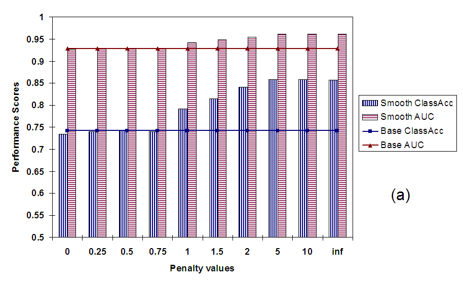
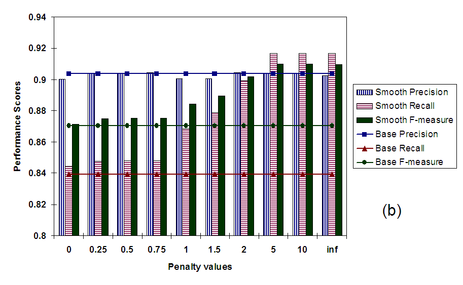
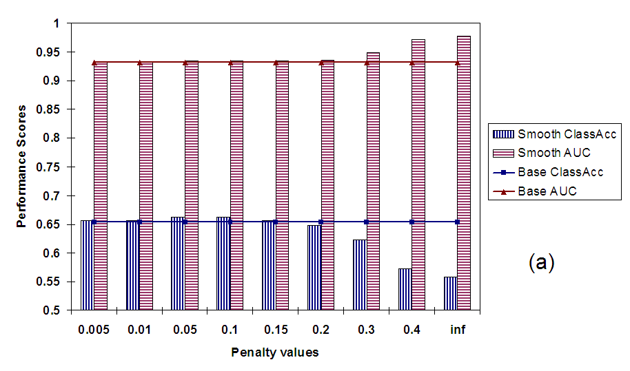
First we discuss the performance of isotonic smoothing in terms of average classification accuracy per class and average AUC per document. In Figure 5(a) we plot both these measures against varying values of penalty. As we vary the penalty from 0 to $\infty$, the problem changes from simple isotonic regression to enforcing the strict monotonicity constraints. We can see from the plots that this progression of problems also translates into improved performance; both classification accuracy and AUC increase significantly with higher penalties. This shows that our method for smoothing classifier scores improves performance from the perspectives of both the classes as well as the documents.

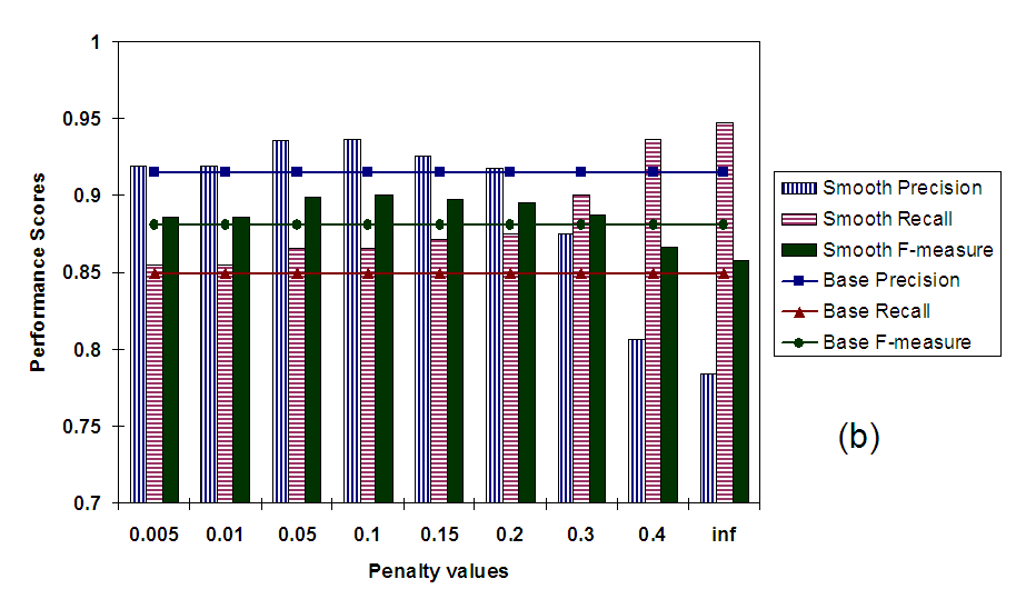
Figure 5(b) plots the values for precision, recall, and F-measure averaged across all documents. Once again, these values are plotted against increasing penalty values. As we can see F-measure rises as penalties are increased and we move towards enforcing strict monotonicity constraints. These strict constraints ensure that the value of the parent is equal to the value of at least one of its children. This type of smoothing takes care of situations where leaf-level classes are mislabeled while their parent nodes are correctly labeled. In these cases, high penalty values make children conform to the parent's score correcting the error, resulting in increased precision and recall. However, strict constraints can also sometime lead to some false positives - especially in shallow hierarchies like the 20-newsgroups - causing a decrease in precision. These trends are exactly what we observe in Figure 5(b). However, the increase in recall compensates for the slight decrease in precision by far, resulting in a higher overall F-measure score.

Since we are evaluating on a dataset that falls under Scenario I, and the strict monotonicity property was framed for just such a scenario, it makes sense that of all penalty values, $\gamma=\infty$ results in best performance. However, it is also interesting to observe the behavior of our dynamic programming based method for low and high range of penalties. As we can see from Figure 5(a) and Figure 5(b) for penalty values between 0 and 1 there is hardly any change in performance from simple isotonic regression ($\gamma=0$). This is because, in this range of penalty the cost to a node for deviating from its parent's smoothed value is less than the cost from $L_1$ error for deviating from its own original value. Hence, the regularization term gets no chance to correct certain types of common errors, especially in shallow hierarchies like TAXONOMYI. Also, as penalty increases well above 1 ( $\gamma \approx 5$) the increase in performance saturates. This is because once penalty becomes sufficiently large it becomes impossible to violate any strict monotonicity constraints (a node's value always equals the maximum of its children's value) and the smoothing behaves as if penalty was set to $\infty$.

We summarize the performance of our smoothing approach in Table 1 and Table 2. As we can see, over and above just classification smoothing provides considerable gains in terms of classification accuracy over classes and precision-recall of labels for a document. According to our results simple isotonic regression without penalties results in almost no improvement highlighting that the gains are due to the regularization aspect our approach.

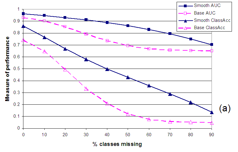
THE EFFECT OF MISSING CLASSIFIER SCORES.

In certain applications, especially those involving dynamic, fast changing, and vast corpora like the Web, we may not have the time or the data to train classifiers for each node (internal or leaf-level) in a hierarchical classification system. In such situations we can classify test instances for nodes with trained classifiers, while resorting to guessing at values for nodes without classifiers. In this section we evaluate whether smoothing the outputs of classifiers that have been trained can help us predict scores for classifiers that haven't been learned.

In order to simulate situations like these we randomly select a set fraction of nodes in our 20-newsgroups taxonomy that we don't train classifiers for. Then we apply our smoothing approach to the tree of nodes (some with missing values) and see if the smoothed scores of the nodes with missing values match the true labels. In our dynamic programming based method the nodes with missing values are given a weight of zero so that they don't contribute to the $L_1$ error. The smoothing approach, hence, replaces the values of the missing nodes with whatever value that helps reduce the cost of isotonic smoothing. However, as the number of missing nodes increases the amount of information provided to the smoothing algorithm decreases and, therefore, we expect the performance of the whole system to also degrade.

In order to provide baseline performance we replace the missing classifier scores randomly with a true or a false - we bias the random predictions by the observed priors for the missing class. This class prior information is gathered from the training data for the class. In situations where classifier values are missing because of lack of training data, we can use other priors for these replacements (maybe average size of other classes in the data). Note that we didn't use the class prior information in the smoothing approach to predicting missing values.

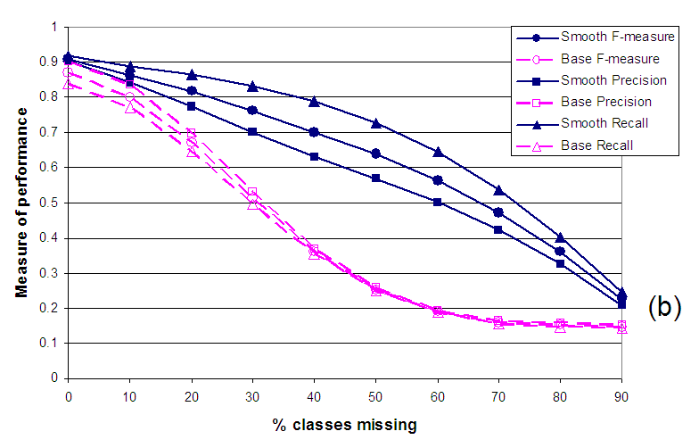
In Figure 6 we examine the performance of our system as the fraction of missing classes is increased (on the X-axis). The performance is measured in terms of the metrics mentioned earlier in this paper. As we can see from the plots, as the fraction of missing values increases the performance decreases. However, the decrease in the quality of smoothed outputs is far lower than the baseline predictions. Even though the smoothed and baseline predictions start with similar accuracy values, the difference between their performances grows dramatically with increasing number of missing values. For instance, in Figure 6(a) the classification accuracy after smoothing is 16% higher than baseline with no missing values and this difference grows to 254% at 50% missing values. Similarly, the corresponding numbers for AUC are 3% and 24%. Figure 6(b) graphs performance in terms of precision, recall, and F-measure against varying amounts of missing values. Once again as the number of missing values increases, the difference in performance of smoothed outputs over baseline balloons: at 50% missing values, smoothing outperforms baseline by 155% in terms of F-measure.

The decrease in performance of baseline predictions is very dramatic at the beginning but after sufficient number of values are missing the effect of predicting with priors kicks in and the accuracy stabilizes. Since our smoothing approach does not use the knowledge of class priors, its performance never stops decreasing and at around 90% missing values the accuracy of smoothed scores and baseline scores is similar again. Hence, devising a well founded way to incorporate such prior information into the smoothing will improve the performance of our approach even more, especially in adverse conditions with many missing values.

Figure 7: Performance with SVMs under Scenario II. With isotonic smoothing (bars). Without smoothing (horizontal lines).

3 Results on TAXONOMYII

In this section we evaluate the performance of our smoothing approach under Scenario II, where documents also belong to internal nodes. Here while smoothing we cannot assume that a node's score must equal the maximum of its children's score. The document being classified may not belong to any of the children and hence a node's score can be larger than all its children's scores. In such a scenario the role of regularization is more subtle than in previous experiments. Very aggressive regularization will enforce strict monotonicity constraints which do not match the problem. Hence, the regularization penalty will have to be large enough to undo classification errors but also low enough to leave room for legitimate cases where documents are not classified into any child.

In fact, we observe exactly this behavior in the plots in Figure 7(a) and Figure 7(a). As we increase the penalty from 0 to $\infty$, the performance measures first increase and then decrease. The only exceptions to this trend of rise and fall are the Recall and AUC measures. Recall increases because as we increase the penalty (and start enforcing strict monotonicity), more children classes are forcefully and erroneously labeled positive. This increase in Recall and AUC is offset by a decrease in Precision and, hence, the F-measure.

These above results showcase a scenario where penalties need to set in a node-specific manner. When we used a standard penalty value for all nodes we didn't see any improvement in performance upon smoothing. This was because the same penalty that lead to correction of an error at a leaf-level class, introduced errors in other cases where a document belonged to an internal node (and not to any of its children). Hence, gains in classification accuracy in one part of the tree were offset by losses in others. Figure 7(a) and Figure 7(a) correspond to experiments in which penalties for nodes were set in proportion to the chance that a document belonging to the node also belongs to one of its children (the value on the X-axis is the proportionality constant). At a given node, the more the chance the higher its penalty value was set, as this ensured that the node's value was close to the maximum of its children's values.

Even with the node-specific penalties, the performance gains at the best values of penalty are very modest: at penalty=0.1, F-measure and Classification Accuracy increase above the baseline by 2% and 1.3% respectively. This is because the hypothesis that we are trying to enforce here is very weak, and many erroneous classifications of a document pass the hypothesis. A stronger property that relates classification scores of adjacent nodes (like in Scenario I) will lead to higher performance gains.

4 Related Work

While we are not aware of any work that explicitly post-processes classifier outputs in a taxonomy in order to correct errors and improve accuracy, in this section we present some existing work on related topics.

HIERARCHICAL TEXT CLASSIFICATION.

Hierarchical classifiers have been used to segment classification problems into more manageable units at the nodes of the hierarchy [3]. Using well defined hierarchies ensures that a smaller set of features suffices for each classifier [6,10]. Dumais et al. [6] work with SVM classifiers on a two-level hierarchy and show that hierarchical classification performs better than classification over a flat set of classes. Similar results are shown by Punera et al. in [14], where the effect of quality of hierarchy on classification accuracy is examined.

EXPLOITING CLASS RELATIONSHIPS IN CLASSIFIER.

The inter-class relationships in hierarchies can be exploited to improve the accuracy of classification. One of the early works in this area employed a statistical technique called shrinkage to improve parameter estimates of nodes in scarce data situations via the estimates of parent nodes [11]. Chakrabarti et al. [4] present Hyperclass, a classifier for webpages that, while classifying a page, consults the labels of its neighboring (hyperlinked) webpages. Finally, there is some recent work on generalizing support vector learning to take into account relationships among classes mirrored in the class-hierarchy [17].

Our work differs from these approaches by exploiting inter class relationships as a post-processing step leaving classifiers to treat each class individually. There are a couple of distinct advantages of this paradigm. First, by separating monotonicity enforcement from classification, we drastically simplify the latter step and can use any off-the-shelf classifier. This way we can take advantage of all the different classifier that have been developed, many of them for specialized domains. Second, while the above classifiers can be trained to follow monotonicity rules there is no guarantee that on a test instance they will produce monotonic outputs, a requirement that might be critical in some domains.

ISOTONIC REGRESSION.

Isotonic regression has been used in many domains such as epidemiology, microarray data analysis [1], webpage cleaning [2], and calibration of classifiers [19]. Similarly, many works have proposed efficient algorithms for finding optimal solutions. For complete orders the optimal solutions can be computed in $O(N\log{N})$ for $L_1$, and $O(N)$ time for $L_2$ distance metrics [16]. For isotonic regression on rooted trees the best known algorithms work in $O(N\log{N})$ time for $L_2$  [13] and $O(N^2\log{N})$ time for $L_1$ metrics [1]. A regularized version of the isotonic regression problem is solved in [2], once again in $O(N^2\log{N})$ time for the $L_1$ metric.

In this paper we have introduced a different isotonic regression problem in which the regularization term only depends on the parent value and the maximum of its children's values. This distinct constraint is motivated by the classifier output smoothing problem. We presented a dynamic programming based method to solve this new problem optimally in $O(N^2\log{N})$ time for the $L_1$ metric.

5 Conclusion and Future Work

In this paper we formulated the problem of smoothing classifier outputs as a novel optimization problem that we call regularized isotonic regression. To solve this problem, we presented an efficient algorithm that gives an optimal solution. Moreover, using a real-world text dataset we showed that performing smoothing as a post-processing step after classification can drastically improve accuracy.

Interesting future work includes applying isotonic smoothing of hierarchical classifiers to other domains (with novel cost functions and constraints), and devising well founded ways to incorporate prior knowledge (like class priors) into the smoothing formulation.

ACKNOWLEDGMENTS. The authors thank Deepayan Chakrabarti and Ravi Kumar for valuable discussions.

Bibliography

1

S. Angelov, B. Harb, S. Kannan, and L.-S. Wang.
Weighted isotonic regression under the L1 norm.
In Proc. of Annual ACM-SIAM Symposium on Discrete Algorithms, pages 783-791, 2006.

2

D. Chakrabarti, R. Kumar, and K. Punera.
Page-level template detection via isotonic smoothing.
In Proc. of International Conference on World Wide Web, pages 61-70. ACM Press, 2007.

3

S. Chakrabarti, B. Dom, R. Agrawal, and P. Raghavan.
Scalable feature selection, classification and signature generation for organizing large text databases into hierarchical topic taxonomies.
VLDB Journal: Very Large Data Bases, 7(3):163-178, 1998.

4

S. Chakrabarti, B. Dom, and P. Indyk.
Enhanced hypertext categorization using hyperlinks.
In Proc. of ACM SIGMOD International Conference on Management of Data, pages 307-318. ACM Press, 1998.

5

DMOZ.
Open directory project, http://www.dmoz.org.

6

S. Dumais and H. Chen.
Hierarchical classification of web content.
In Proc. of Annual International ACM Conference on Research and Development in Information Retrieval, pages 256-263. ACM Press, 2000.

7

T. Fawcett.
ROC graphs: Notes and practical considerations for data mining researchers.
Technical Report HPL-2003-4, Hewlett Packard Laboratories, Jan. 17 2003.

8

T.-K. Huang, R. C. Weng, and C.-J. Lin.
Generalized Bradley-Terry models and multi-class probability estimates.
Journal of Machine Learning Research, 7:85-115, 2006.

9

T. Joachims.
Text categorization with support vector machines: learning with many relevant features.
In Proc. of European Conference on Machine Learning, pages 137-142, 1998.

10

D. Koller and M. Sahami.
Hierarchically classifying documents using very few words.
In Proc. of International Conference on Machine Learning, pages 170-178. Morgan Kaufmann Publishers Inc., 1997.

11

A. McCallum, R. Rosenfeld, T. M. Mitchell, and A. Y. Ng.
Improving text classification by shrinkage in a hierarchy of classes.
In Proc. of International Conference on Machine Learning, pages 359-367. Morgan Kaufmann Publishers Inc., 1998.

12

T. Mitchell.
Machine Learning.
McGraw Hill, 1997.

13

P. M. Pardalos and G. Xue.
Algorithms for a class of isotonic regression problems.
Algorithmica, 23(3):211-222, 1999.

14

K. Punera, S. Rajan, and J. Ghosh.
Automatic construction of n-ary tree based taxonomies.
In Proc. of IEEE International Conference on Data Mining - Workshops, pages 75-79. IEEE Computer Society, 2006.

15

J. Rennie and R. Rifkin.
Improving multiclass text classification with the support vector machine.
AI Memo AIM-2001-026, Massachusetts Institute of Technology, 2001.

16

Q. Stout.
Optimal algorithms for unimodal regression.
Computing Science and Statistics, 32:348-355, 2000.

17

I. Tsochantaridis, T. Joachims, T. Hofmann, and Y. Altun.
Large margin methods for structured and interdependent output variables.
Journal of Machine Learning Research, 6:1453-1484, 2005.

18

Yahoo!
Web directory http://dir.yahoo.com.

19

B. Zadrozny and C. Elkan.
Transforming classifier scores into accurate multiclass probability estimates.
In Proc. of ACM SIGKDD International Conference on Knowledge Discovery and Data Mining, pages 694-699, 2002.

Footnotes

... classes¹

Our formulations and algorithms also hold for setting where an instance belongs to more than one leaf-level nodes.

... dataset²

http://people.csail.mit.edu/jrennie/20Newsgroups/