Large-Scale Text Categorization by
Batch Mode Active Learning
Abstract:
Large-scale text categorization is an important research topic for
Web data mining. One of the challenges in large-scale text
categorization is how to reduce the human efforts in labeling text
documents for building reliable classification models. In the
past, there have been many studies on applying active learning
methods to automatic text categorization, which try to select the
most informative documents for labeling manually. Most of these
studies focused on selecting a single unlabeled document in
each iteration. As a result, the text categorization model has to
be retrained after each labeled document is solicited. In this
paper, we present a novel active learning algorithm that selects a
batch of text documents for labeling manually in each
iteration. The key of the batch mode active learning is how to
reduce the redundancy among the selected examples such that each
example provides unique information for model updating. To this
end, we use the Fisher information matrix as the measurement of
model uncertainty and choose the set of documents to effectively
maximize the Fisher information of a classification model.
Extensive experiments with three different datasets have shown
that our algorithm is more effective than the state-of-the-art
active learning techniques for text categorization and can be a
promising tool toward large-scale text categorization for World
Wide Web documents.
H.3.3Information Systems Information Search and
Retrieval I.5.2 Design Methodology Classifier Design
and Evaluation
Algorithms, Performance, Experimentation
text categorization, active learning, logistic regression,
Fisher information, convex optimization
The goal of text categorization is to automatically assign text
documents to the predefined categories. With the rapid growth of Web
pages on the World Wide Web (WWW), text categorization has become
more and more important in both the world of research and
applications. Usually, text categorization is regarded as a
supervised learning problem. In order to build a reliable model for
text categorization, we need to first of all manually label a number
of documents using the predefined categories. Then, a statistical
machine learning algorithm is engaged to learn a text classification
model from the labeled documents. One important challenge for
large-scale text categorization is how to reduce the number of
labeled documents that are required for building reliable text
classification models. This is particularly important for text
categorization of WWW documents given its large size.
To reduce the number of labeled documents, in the past, there have
been a number of studies on applying active learning to text
categorization. The main idea is to only select the most
informative documents for labeling manually. Most active learning
algorithms are conducted in the iterative fashion. In each
iteration, the example with the largest classification uncertainty
is chosen for labeling manually. Then, the classification model is
retrained with the additional labeled example. The step of
training a classification model and the step of soliciting a
labeled example are iterated alternatively until most of the
examples can be classified with reasonably high confidence. One of
the main problems with such a scheme is that only a single
example is selected for labeling. As a result, the classification
model has to be retrained after each labeled example is solicited.
In the paper, we propose a novel active learning scheme that is able
to select a batch of unlabeled examples in each iteration. A
simple strategy toward the batch mode active learning is to select
the top  most informative examples. The problem with such an
approach is that some of the selected examples could be similar, or
even identical, and therefore do not provide additional information
for model updating. In general, the key of the batch mode active
learning is to ensure the small redundancy among the selected
examples such that each example provides unique information for
model updating. To this end, we use the Fisher information matrix,
which represents the overall uncertainty of a classification model.
We choose the set of examples such that the Fisher information of a
classification model can be effectively maximized.
most informative examples. The problem with such an
approach is that some of the selected examples could be similar, or
even identical, and therefore do not provide additional information
for model updating. In general, the key of the batch mode active
learning is to ensure the small redundancy among the selected
examples such that each example provides unique information for
model updating. To this end, we use the Fisher information matrix,
which represents the overall uncertainty of a classification model.
We choose the set of examples such that the Fisher information of a
classification model can be effectively maximized.
The rest of this paper is organized as follows.
Section 2 reviews the related work on text
categorization and active learning algorithms. Section 3
briefly introduces the concept of logistic regression, which is used
as the classification model in our study for text categorization.
Section 4 presents the batch mode active learning
algorithm and an efficient learning algorithm based on the bound
optimization algorithm. Section 5 presents the results
of our empirical study. Section 6 sets out our
conclusions.
2 Related Work
Text categorization is a long-term research topic which has been
actively studied in the communities of Web data mining, information
retrieval and statistical learning [15,35].
Essentially the text categorization techniques have been the key
toward automated categorization of large-scale Web pages and Web
sites [18,27], which is further applied to improve
Web searching engines in finding relevant documents and to
facilitate users in browsing Web pages or Web sites.
In the past decade, a number of statistical learning techniques
have been applied to text categorization [34], including
the K Nearest Neighbor approaches [20], decision
trees [2], Bayesian
classifiers [32], inductive rule
learning [5], neural
networks [23], and support vector machines
(SVM) [9]. Empirical studies in recent
years [9] have shown that SVM is the
state-of-the-art technique among all the methods mentioned above.
Recently, logistic regression, a traditional statistical tool, has
attracted considerable attention for text categorization and
high-dimension data mining [12]. Several recent
studies have shown that the logistic regression model can achieve
comparable classification accuracy as SVMs in text categorization.
Compared to SVMs, the logistic regression model has the advantage
in that it is usually more efficient than SVMs in model training,
especially when the number of training documents is
large [13,36]. This motivates us to choose
logistic regression as the basis classifier for large-scale text
categorization.
The other critical issue for large-scale text document
categorization is how to reduce the number of labeled documents
that are required for building reliable text classification
models. Given the limited amount of labeled documents, the key is
to exploit the unlabeled documents. One solution is the
semi-supervised learning, which tries to learn a classification
model from the mixture of labeled and unlabeled
examples [30]. A comprehensive study of
semi-supervised learning techniques can be found in
[25,38]. Another solution is active learning
[19,26] that tries to choose the most
informative unlabeled examples for labeling manually. Although
previous studies have shown the promising performance of
semi-supervised learning for text categorization
[11], the high computation cost has limited its
application [38]. In this paper, we focus our
discussion on active learning.
Active learning, or called pool-based active learning, has been
extensively studied in machine learning for many years and has
already been employed for text categorization in the
past [16,17,21,22]. Most
active learning algorithms are conducted in the iterative fashion.
In each iteration, the example with the highest classification
uncertainty is chosen for labeling manually. Then, the
classification model is retrained with the additional labeled
example. The step of training a classification model and the step
of soliciting a labeled example are iterated alternatively until
most of the examples can be classified with reasonably high
confidence. One of the key issues in active learning is how to
measure the classification uncertainty of unlabeled examples. In
[6,7,8,14,21,26],
a number of distinct classification models are first generated.
Then, the classification uncertainty of a test example is measured
by the amount of disagreement among the ensemble of classification
models in predicting the labels for the test example. Another
group of approaches measure the classification uncertainty of a
test example by how far the example is away from the
classification boundary (i.e., classification margin)
[4,24,31]. One of the most
well-known approaches within this group is support vector
machine active learning developed by Tong and
Koller [31]. Due to its popularity and success in
the previous studies, it is used as the baseline approach in our
study.
One of the main problems with most existing active learning
algorithm is that only a single example is selected for
labeling. As a result, the classification model has to be retrained
after each labeled example is solicited. In this paper, we focus on
the batch mode active learning that selects a batch of
unlabeled examples in each iteration. A simple strategy is to choose
the top most uncertain examples. However, it is likely that some
of the most uncertain examples can be strongly correlated and even
identical in the extreme cases, which are redundant in providing the
informative clues to the classification model. In general, the
challenge in choosing a batch of unlabeled examples is twofold: on
one hand the examples in the selected batch should be informative to
the classification model; on the other hand the examples should be
diverse enough such that information provided by different examples
does not overlap with each other. To address this challenge, we
employ the Fisher information matrix as the measurement of model
uncertainty, and choose the set of examples that efficiently
maximize the Fisher information of the classification model. Fisher
information matrix has been used widely in statistics for measuring
model uncertainty [28]. For example, in the Cramer-Rao
bound, Fisher information matrix provides the low bound for the
variance of a statistical model. In this study, we choose the set of
examples that can well represent the structure of the Fisher
information matrix.
3 Logistic Regression
In this section, we give a brief background review of logistic
regression, which has been a well-known and mature statistical
model suitable for probabilistic binary classification. Recently,
logistic regression has been actively studied in statistical
machine learning community due to its close relation to SVMs and Adaboost [33,36].Compared with many other statistical learning models, such as
SVMs, the logistic regression model has the following advantages:
- It is a high performance classifier that can be efficiently
trained with a large number of labeled examples. Previous studies
have shown that the logistic regression model is able to achieve
the similar performance of text categorization as
SVMs [13,36]. These studies also showed that the
logistic regression model can be trained significantly more
efficiently than SVMs, particularly when the number of labeled
documents is large.
- It is a robust classifier that does not have any configuration parameters to tune.
In contrast, some state-of-the-art classifiers, such as support
vector machines and AdaBoost, are sensitive to the setup of the
configuration parameters. Although this problem can be partially
solved by the cross validation method, it usually introduces a
significant amount of overhead in computation.
Logistic regression can be applied to both real and binary data.
It outputs the posterior probabilities for test examples that can
be conveniently processed and engaged in other systems. In theory,
given a test example  , logistic regression models the conditional
probability of assigning a class label
, logistic regression models the conditional
probability of assigning a class label  to the example by
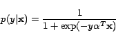 |
(1) |
where
 , and
, and  is the model parameter. Here
a bias constant is omitted for simplified
notation. In general, logistic regression is a linear classifier that has
been shown effective in classifying text documents that are
usually in the high-dimensional data space. For the implementation
of logistic regressions, a number of efficient algorithms have
been developed in the recent literature [13].
is the model parameter. Here
a bias constant is omitted for simplified
notation. In general, logistic regression is a linear classifier that has
been shown effective in classifying text documents that are
usually in the high-dimensional data space. For the implementation
of logistic regressions, a number of efficient algorithms have
been developed in the recent literature [13].
4 Batch Mode Active Learning
In this section, we present a batch mode active learning algorithm
for large-scale text categorization. In our proposed scheme,
logistic regression is used as the base classifier for binary
classification. In the following, we first introduce the
theoretical foundation of our active learning algorithm. Based on
the theoretical framework, we then formulate the active learning
problem into a semi-definite programming (SDP)
problem [3]. Finally, we present an efficient learning
algorithm for the related optimization problem based on the eigen
space simplification and a bound optimization strategy.
Our active learning methodology is motivated by the work
in [37], in which the author presented a theoretical
framework of active learning based on the Fisher information matrix.
Given the Fisher information matrix represents the overall
uncertainty of a classification model, our goal is to search for a
set of examples that can most efficiently maximize the Fisher
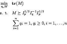
information. As showed in [37], this goal can be
formulated into the following optimization problem:
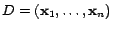
Let  be the distribution of all unlabeled examples,
and
be the distribution of all unlabeled examples,
and  be the distribution of unlabeled examples that
are chosen for labeling manually. Let denote the
parameters of the classification model. Let
be the distribution of unlabeled examples that
are chosen for labeling manually. Let denote the
parameters of the classification model. Let  and
and
 denote the Fisher information matrix of the
classification model for the distribution and
, respectively. Then, the set of examples that can
most efficiently reduce the uncertainty of classification model is
found by minimizing the ratio of the two Fisher information matrix
and , i.e.,
denote the Fisher information matrix of the
classification model for the distribution and
, respectively. Then, the set of examples that can
most efficiently reduce the uncertainty of classification model is
found by minimizing the ratio of the two Fisher information matrix
and , i.e.,
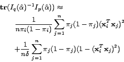
For the logistic regression model, the Fisher information
is attained as:
 |
(3) |
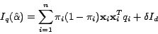
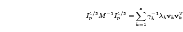
In order to estimate the optimal distribution , we
replace the integration in the above equation with the summation
over the unlabeled data, and the model parameter with the
empirically estimated  . Let
. Let
 be the unlabeled data. We can
now rewrite the above expression for Fisher information matrix as:
be the unlabeled data. We can
now rewrite the above expression for Fisher information matrix as:
 |
(4) |
where
 |
(5) |
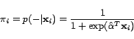
In the above,  stands for the probability of selecting the
 -th example and is subjected to
 ,
,  is the identity matrix of
  dimension, and
  is the
smoothing parameter. The
is the
smoothing parameter. The  term is added to the
estimation of
term is added to the
estimation of
 to prevent it from being a
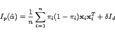
singular matrix. Similarly, for
to prevent it from being a
singular matrix. Similarly, for
 , the Fisher
information matrix for all the unlabeled examples, we have it
expressed as follows:
, the Fisher
information matrix for all the unlabeled examples, we have it
expressed as follows:
 |
(6) |
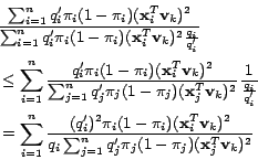
In this section, we will qualitatively justify the theory of
minimizing the Fisher information for batch mode active learning.
In particular, we consider two cases, the case of selecting a
single unlabeled example and the case of selecting two unlabeled
examples simultaneously. To simplify our discussion, let's assume
 for all unlabeled examples.
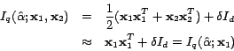
Selecting a single unlabeled example. The Fisher information
matrix  is simplified into the following form when the -th
example is selected:
is simplified into the following form when the -th
example is selected:
Then, the objective function
 becomes:
To minimize the above expression, we need to maximize the term
 , which reaches its maximum value at
  . Since
 , the value of
can be regarded as the measurement of
classification uncertainty for the -th unlabeled example. Thus,
the optimal example chosen by minimizing the Fisher information
matrix in the above expression tends to be the one with a high
classification uncertainty.
, the value of
can be regarded as the measurement of
classification uncertainty for the -th unlabeled example. Thus,
the optimal example chosen by minimizing the Fisher information
matrix in the above expression tends to be the one with a high
classification uncertainty.
Selecting two unlabeled examples simultaneously. To simplify
our discussion, we assume that the three examples,  ,
,
 , and
, and  , have the largest classification
uncertainty. Let's further assume that
, have the largest classification
uncertainty. Let's further assume that
 , and meanwhile is far away from
and . Then, if we follow the simple
greedy approach, the two example and
will be selected given their largest classification uncertainty.
Apparently, this is not an optimal strategy given both examples
provide almost identical information for updating the classification
model. Now, if we follow the criterion of minimizing Fisher
information, this mistake could be prevented because
, and meanwhile is far away from
and . Then, if we follow the simple
greedy approach, the two example and
will be selected given their largest classification uncertainty.
Apparently, this is not an optimal strategy given both examples
provide almost identical information for updating the classification
model. Now, if we follow the criterion of minimizing Fisher
information, this mistake could be prevented because
As indicated in the above equation, by including the second example
, we did not change the expression of , the
Fisher information matrix for the selected examples. As a result,
there will be no reduction in the objective function
 when including
the example . Instead, we may want to choose
that is more likely to decrease the objective
function even though its classification uncertainty is smaller than
that of .
when including
the example . Instead, we may want to choose
that is more likely to decrease the objective
function even though its classification uncertainty is smaller than
that of .
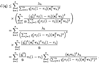
The idea of our batch mode active learning approach is to search a
distribution  that minimizes
 . The
samples with maximum values of will then be chosen for
queries. However, it is usually not easy to find an appropriate
distribution that minimizes
. In
the following, we present a semidefinite programming (SDP) approach
for optimizing
.
. The
samples with maximum values of will then be chosen for
queries. However, it is usually not easy to find an appropriate
distribution that minimizes
. In
the following, we present a semidefinite programming (SDP) approach
for optimizing
.
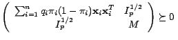
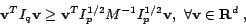
Given the optimization problem in (2), we can rewrite
the objective function
as
 . We then introduce a
slack matrix
. We then introduce a
slack matrix
 such that
 . Then original optimization problem can
be rewritten as follows:
. Then original optimization problem can
be rewritten as follows:
 |
(7) |
In the above, we use the property
 if
if  . Furthermore, we use the Schur
complementary, i.e.,
. Furthermore, we use the Schur
complementary, i.e.,
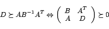 |
(8) |
if  . This will lead to the following formulation of
the problem in (7)
. This will lead to the following formulation of
the problem in (7)
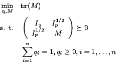 |
(9) |
or more specifically
The above problem belongs to the family of Semi-definite programming
and can be solved by the standard convex optimization packages such
as SeDuMi [29].
Although the formulation in (10) is mathematically
sound, directly solving the optimization problem could be
computationally expensive due to the large size of matrix  ,
i.e.,
,
i.e.,  , where is the dimension of data. In order to
reduce the computational complexity, we assume that is only
expanded in the eigen space of matrix
, where is the dimension of data. In order to
reduce the computational complexity, we assume that is only
expanded in the eigen space of matrix 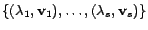 . Let
. Let
 be the top
 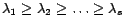 eigen vectors of matrix where
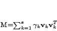 . We assume matrix has the following
form:
. We assume matrix has the following
form:
 |
(13) |
where the combination parameters
 . We
rewrite the inequality for
as
. We
rewrite the inequality for
as
 . Using the expression for
in (11), we have
. Using the expression for
in (11), we have
 |
(14) |
Given that the necessary condition for
is
we have
 for
for  . This necessary condition leads to following
constraints for
. This necessary condition leads to following
constraints for 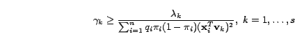 :
:
Meanwhile, the objective function in (10) can be
expressed as
 |
(15) |
By putting the above two expressions together, we transform the SDP
problem in (10) into the following optimization problem:
 |
(17) |
Note that the above optimization problem is a convex optimization
problem since  is convex when
  . In the next
subsection, we present a bound optimization algorithm for solving
the optimization problem in (15).
. In the next
subsection, we present a bound optimization algorithm for solving
the optimization problem in (15).
The main idea of bound optimization algorithm is to update the
solution iteratively. In each iteration, we will first calculate the
difference between the objective function of the current iteration
and the objective function of the previous iteration. Then, by
minimizing the upper bound of the difference, we find the solution
of the current iteration.
Let  and
and  denote the solutions obtained in
two consecutive iterations, and let
denote the solutions obtained in
two consecutive iterations, and let
 be the
objective function in (15). Based on the proof given in
Appendix-A, we have the following expression:
be the
objective function in (15). Based on the proof given in
Appendix-A, we have the following expression:
Now, instead of optimizing the original objective function
, we can optimize its upper bound, which
leads to the following simple updating equation:
 |
(19) |
Similar to all bound optimization algorithms [3], this
algorithm will guarantee to converge to a local maximum. Since the
original optimization problem in (15) is a convex
optimization problem, the above updating procedure will guarantee to
converge to a global optimal.
Remark: It is interesting to examine the property of the
solution obtained by the updating equation in (17).
First, according to (17), the example with a large
classification uncertainty will be assigned with a large
probability. This is because is proportional to
, the classification uncertainty of the -the unlabeled
example. Second, according to (17), the example that
is similar to many unlabeled examples is more likely to be
selected. This is because probability is proportional to the
term
 , the similarity of the -th
example to the principal eigenvectors. This is consistent with our
intuition that we should select the most informative and
representative examples for active learning.
, the similarity of the -th
example to the principal eigenvectors. This is consistent with our
intuition that we should select the most informative and
representative examples for active learning.
5 Experimental Results
Table 1:
A list of  major categories of the Reuters-21578
dataset in our experiments.
major categories of the Reuters-21578
dataset in our experiments.
| Category |
# of total samples |
| earn |
3964 |
| acq |
2369 |
| money-fx |
717 |
| grain |
582 |
| crude |
578 |
| trade |
485 |
| interest |
478 |
| wheat |
283 |
| ship |
286 |
| corn |
237 |
|
Table 2:
A list of  categories of the WebKB dataset in our experiments.
| Category |
# of total samples |
| course |
930 |
| department |
182 |
| faculty |
1124 |
| project |
504 |
| staff |
137 |
| student |
1641 |
|
Table 3:
A list of  categories of the Newsgroup dataset in our experiments.
| Category |
# of total samples |
| 0 |
1000 |
| 1 |
1000 |
| 2 |
1000 |
| 3 |
1000 |
| 4 |
1000 |
| 5 |
1000 |
| 6 |
999 |
| 7 |
1000 |
| 8 |
1000 |
| 9 |
1000 |
| 10 |
997 |
|
In this section we discuss the experimental evaluation of our active
learning algorithm in comparison to the state-of-the-art approaches.
For a consistent evaluation, we conduct our empirical comparisons on
three standard datasets for text document categorization. For all
three datasets, the same pre-processing procedure is applied: the
stopwords and the numbers are removed from the documents, and all
the words are converted into the low cases without stemmming.
The first dataset is the Reuters-21578 Corpus dataset, which has
been widely used as a testbed for evaluating algorithms for text
categorization. In our experiments, the ModApte split of the
Reuters-21578 is used. There are a total of  text documents
in this collection. Table 1 shows a list of the
most frequent categories contained in the dataset. Since each
document in the dataset can be assigned to multiple categories, we
treat the text categorization problem as a set of binary
classification problems, i.e., a different binary classification
problem for each category. In total,
text documents
in this collection. Table 1 shows a list of the
most frequent categories contained in the dataset. Since each
document in the dataset can be assigned to multiple categories, we
treat the text categorization problem as a set of binary
classification problems, i.e., a different binary classification
problem for each category. In total,  word features are
extracted and used to represent the text documents.
word features are
extracted and used to represent the text documents.
The other two datasets are Web-related: the WebKB data collection
and the Newsgroup data collection. The WebKB dataset comprises of
the WWW-pages collected from computer science departments of
various universities in January 1997 by the World Wide Knowledge
Base (Web- Kb) project of the CMU text learning group. All the
Web pages are classified into seven categories: student, faculty,
staff, department, course, project, and other. In this study, we
ignore the category of others due to its unclear definition. In
total, there are
Kb) project of the CMU text learning group. All the
Web pages are classified into seven categories: student, faculty,
staff, department, course, project, and other. In this study, we
ignore the category of others due to its unclear definition. In
total, there are  data samples in the selected dataset, and
 word features are extracted to represent the text
documents. Table 2 shows the details of this
dataset. The newsgroup dataset includes
word features are extracted to represent the text
documents. Table 2 shows the details of this
dataset. The newsgroup dataset includes  messages from
 different newsgroups. Each newsgroup contains roughly about
 messages. In this study, we randomly select out of 20
newsgroups for evaluation. In total, there are
messages. In this study, we randomly select out of 20
newsgroups for evaluation. In total, there are  data
samples in the selected dataset, and
data
samples in the selected dataset, and  word features are
extracted to represent the text documents.
Table 3 shows the details of the engaged dataset.
word features are
extracted to represent the text documents.
Table 3 shows the details of the engaged dataset.
Compared to the Reuter-21578 dataset, the two Web-related data
collections are different in that more unique words are found in
the Web-related datasets. For example, for both the Reuter-21578
dataset and the Newsgroup dataset, they both contain roughly
 documents. But, the number of unique words for the
Newgroups dataset is close to
documents. But, the number of unique words for the
Newgroups dataset is close to  , which is about twice as
the number of unique words found in the Reuter-21578. It is this
feature that makes the text categorization of WWW documents more
challenging than the categorization of normal text documents
because considerably more feature weights need to be decided for
the WWW documents than the normal documents. It is also this
feature that makes the active learning algorithms more valuable
for text categorization of WWW documents than the normal documents
since by selecting the informative documents for labeling
manually, we are able to decide the appropriate weights for more
words than by a randomly chosen document.
, which is about twice as
the number of unique words found in the Reuter-21578. It is this
feature that makes the text categorization of WWW documents more
challenging than the categorization of normal text documents
because considerably more feature weights need to be decided for
the WWW documents than the normal documents. It is also this
feature that makes the active learning algorithms more valuable
for text categorization of WWW documents than the normal documents
since by selecting the informative documents for labeling
manually, we are able to decide the appropriate weights for more
words than by a randomly chosen document.
In order to remove the uninformative word features, feature
selection is conducted using the Information
Gain [35] criterion. In particular,  of the
most informative features are selected for each category in each of
the three datasets above.
of the
most informative features are selected for each category in each of
the three datasets above.
For performance measurement, the 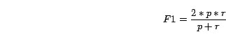 metric is adopted as our
evaluation metric, which has been shown to be more reliable metric
than other metrics such as the classification
accuracy [35]. More specifically, the is
defined as
metric is adopted as our
evaluation metric, which has been shown to be more reliable metric
than other metrics such as the classification
accuracy [35]. More specifically, the is
defined as
 |
(20) |
where  and
and  are precision and recall. Note
that the metric takes into account both the precision and the
recall, thus is a more comprehensive metric than either the
precision or the recall when separately considered.
are precision and recall. Note
that the metric takes into account both the precision and the
recall, thus is a more comprehensive metric than either the
precision or the recall when separately considered.
To examine the effectiveness of the proposed active learning
algorithm, two reference models are used in our experiment. The
first reference model is the logistic regression active learning
algorithm that measures the classification uncertainty based on the
entropy of the distribution
 . In particular, for a
given test example and a logistic regression model with
the weight vector
. In particular, for a
given test example and a logistic regression model with
the weight vector  and the bias term
  , the entropy of
the distribution
is calculated as:
, the entropy of
the distribution
is calculated as:
The larger the entropy of is, the more uncertain we
are about the class labels of . We refer to this
baseline model as the logistic regression active learning, or
LogReg-AL for short. The second reference model is based on
support vector machine [31] that is already
discussed in Section 2 of related work. In
this method, the classification uncertainty of an example
is determined by its distance to the decision
boundary
 , i.e.,
The smaller the distance
 is, the
more the classification uncertainty will be. We refer to this
approach as support vector machine active learning, or
SVM-AL for short. Finally, both the logistic regression model and
the support vector machine that are trained only over the labeled
examples are used in our experiments as the baseline models. By
comparing with these two baseline models, we are able to determine
the amount of benefits that are brought by different active
learning algorithms.
is, the
more the classification uncertainty will be. We refer to this
approach as support vector machine active learning, or
SVM-AL for short. Finally, both the logistic regression model and
the support vector machine that are trained only over the labeled
examples are used in our experiments as the baseline models. By
comparing with these two baseline models, we are able to determine
the amount of benefits that are brought by different active
learning algorithms.
To evaluate the performance of the proposed active learning
algorithms, we first pick  training samples, which include
 positive examples and negative examples, randomly from
the dataset for each category. Both the logistic regression model
and the SVM classifier are trained on the labeled data. For the
active learning methods, unlabeled data samples are chosen
for labeling and their performances are evaluated after rebuilding
the classifiers respectively. Each experiment is carried out
positive examples and negative examples, randomly from
the dataset for each category. Both the logistic regression model
and the SVM classifier are trained on the labeled data. For the
active learning methods, unlabeled data samples are chosen
for labeling and their performances are evaluated after rebuilding
the classifiers respectively. Each experiment is carried out  times and the averaged with its variance is calculated and
used for final evaluation.
times and the averaged with its variance is calculated and
used for final evaluation.
To deploy efficient implementations of our scheme toward
large-scale text categorization tasks, all the algorithms used in
this study are programmed in the C language. The testing hardware
environment is on a Linux workstation with  GHz CPU and
  physical memory. To implement the logistic regression algorithm
for our text categorization tasks, we employ the implementation of
the logistic regression tool developed by Komarek and Moore
recently [13]. To implement our active learning
algorithm based on the bound optimization approach, we employ a
standard math package, i.e., LAPACK [1], to solve
the eigen decomposition in our algorithm efficiently. The
physical memory. To implement the logistic regression algorithm
for our text categorization tasks, we employ the implementation of
the logistic regression tool developed by Komarek and Moore
recently [13]. To implement our active learning
algorithm based on the bound optimization approach, we employ a
standard math package, i.e., LAPACK [1], to solve
the eigen decomposition in our algorithm efficiently. The
 package [10] is used in our
experiments for the implementation of SVM, which has been
considered as the state-of-the-art tool for text categorization.
Since SVM is not parameter-free and can be very sensitive to the
capacity parameter, a separate validation set is used to determine
the optimal parameters for configuration.
package [10] is used in our
experiments for the implementation of SVM, which has been
considered as the state-of-the-art tool for text categorization.
Since SVM is not parameter-free and can be very sensitive to the
capacity parameter, a separate validation set is used to determine
the optimal parameters for configuration.
In this subsection, we will first describe the results for the
Reuter-21578 dataset since this dataset has been most extensively
studied for text categorization. We will then provide the
empirical results for the two Web-related datasets.
Table 4:
Experimental results of F1 performance on the Reuters-21578 dataset with training samples (%).
| Category |
SVM |
LogReg |
SVM-AL |
LogReg-AL |
LogReg-BMAL |
| earn |
92.12  0.22 0.22 |
92.47 0.13 |
93.30 0.28 |
93.40 0.14 |
94.00 0.09 |
| acq |
83.56 0.26 |
83.35 0.26 |
85.96 0.34 |
86.57 0.32 |
88.07 0.17 |
| money-fx |
64.06 0.60 |
63.71 0.63 |
73.32 0.38 |
71.21 0.61 |
75.54 0.26 |
| grain |
60.87 1.04 |
58.97 0.91 |
74.95 0.42 |
74.82 0.53 |
77.77 0.27 |
| crude |
67.78 0.39 |
67.32 0.48 |
75.72 0.24 |
74.97 0.44 |
78.04 0.14 |
| trade |
52.64 0.46 |
48.93 0.55 |
66.41 0.33 |
66.31 0.33 |
69.29 0.34 |
| interest |
56.80 0.60 |
53.59 0.60 |
67.20 0.39 |
66.15 0.49 |
68.71 0.37 |
| wheat |
62.71 0.72 |
57.38 0.79 |
86.01 1.04 |
86.49 0.27 |
88.15 0.21 |
| ship |
67.11 1.59 |
64.91 1.75 |
75.86 0.53 |
72.82 0.46 |
76.82 0.34 |
| corn |
44.39 0.84 |
41.15 0.69 |
71.27 0.62 |
71.61 0.60 |
74.35 0.47 |
|
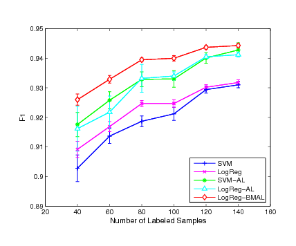
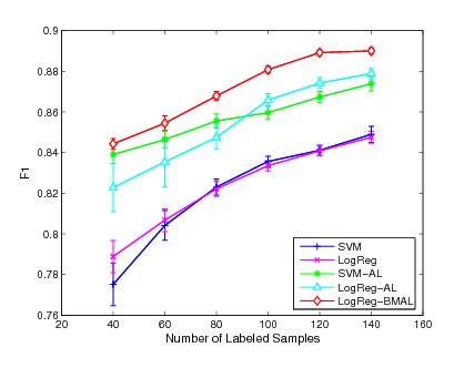
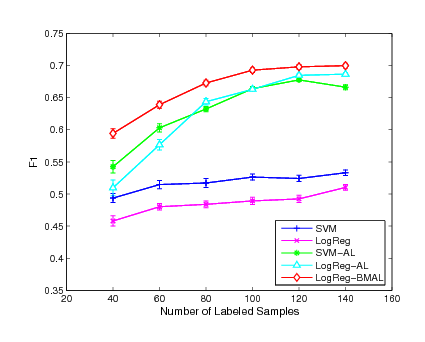
Figure 1:
Experimental results of F1 performance on
the ``earn", ``acq" and ``money-fx" categories
|
|
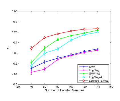
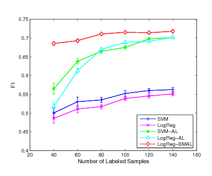
Figure 2:
Experimental results of F1 performance on
the ``grain", ``crude" and ``trade" categories
|
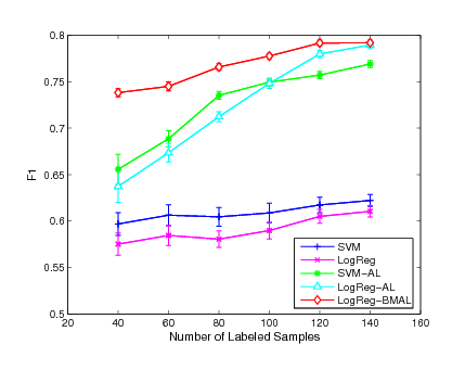
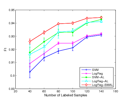
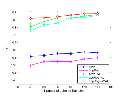
Figure 3:
Experimental results of F1 performance on
the ``interest", ``wheat" and ``ship" categories
|
|
Table 4 shows the experimental results of
performance averaging over executions on major
categories in the dataset.
First, as listed in the first and the second columns of Table
4, we observe that the performance of the
two classifiers, logistic regression and SVM, are comparable when
only the initially labeled examples are used for training.
For categories, such as ``trade'' and ''interest'', SVM achieves
noticeably better performance than the logistic regression model.
Second, we compare the performance of the two classifiers for
active learning, i.e., LogReg-AL and SVM-AL, which are the greedy
algorithms and select the most informative examples for labeling
manually.
The results are listed in
the third and the fourth columns of Table 4.
We find that the performance of these two active learning methods
becomes closer than the case when no actively labeled examples are
used for training. For example, for category ``trade'', SVM performs
substantially better than the logistic regression model when only
labeled examples are used. The difference in measurement
between LogReg-AL and SVM-AL almost diminishes when both classifiers
use the actively labeled examples for training. Finally, we
compare the performance of the proposed active learning algorithm,
i.e., LogReg-BMAL, to the margin-based active learning approaches
LogReg-AL and SVM-AL. It is evident that the proposed batch mode
active learning algorithm outperforms the margin-based active
learning algorithms. For categories, such as ``corn'' and ``wheat'',
where the two margin-based active learning algorithms achieve
similar performance, the proposed algorithm LogReg-BMAL is able to
achieve substantially better scores. Even for the categories
where the SVM performs substantially better than the logistic
regression model, the proposed algorithm is able to outperform the
SVM-based active learning algorithm noticeably. For example, for
category ``ship'' where SVM performs noticeably better than the
logistic regression, the proposed active learning method is able to
achieve even better performance than the margin-based active
learning based on the SVM classifier.
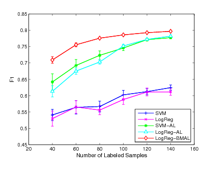
In order to evaluate the performance in more detail, we conduct the
evaluation on each category by varying the number of initially
labeled instances for each classifier. Fig. 1,
Fig. 2 and Fig. 3 show the
experimental results of the mean measurement on  major
categories. From the experimental results, we can see that our
active learning algorithm outperforms the other two active learning
algorithms in most of the cases while the SVM-AL method is generally
better than the LogReg-AL method. We also found that the improvement
of our active learning method is more evident comparing with the
other two approaches when the number of labeled instances is
smaller. This is because the smaller the number of initially labeled
examples used for training, the larger the improvement we would
expect. When more labeled examples are used for training, the gap
for future improvement begins to decrease. As a result, the three
methods start to behavior similarly. This result also indicates that
the proposed active learning algorithm is robust even when the
number of labeled examples is small while the other two active
learning approaches may suffer critically when the margin criterion
is not very accurate for the small sample case.
major
categories. From the experimental results, we can see that our
active learning algorithm outperforms the other two active learning
algorithms in most of the cases while the SVM-AL method is generally
better than the LogReg-AL method. We also found that the improvement
of our active learning method is more evident comparing with the
other two approaches when the number of labeled instances is
smaller. This is because the smaller the number of initially labeled
examples used for training, the larger the improvement we would
expect. When more labeled examples are used for training, the gap
for future improvement begins to decrease. As a result, the three
methods start to behavior similarly. This result also indicates that
the proposed active learning algorithm is robust even when the
number of labeled examples is small while the other two active
learning approaches may suffer critically when the margin criterion
is not very accurate for the small sample case.
Table 5:
Experimental results of F1 performance on the WebKB dataset with training samples (%).
| Category |
SVM |
LogReg |
SVM-AL |
LogReg-AL |
LogReg-BMAL |
| course |
87.11 0.51 |
89.16 0.45 |
88.55 0.48 |
89.37 0.65 |
90.99 0.39 |
| department |
67.45 1.36 |
68.92 1.39 |
82.02 0.47 |
79.22 1.14 |
81.52 0.46 |
| faculty |
70.84 0.76 |
71.50 0.59 |
75.59 0.65 |
73.66 1.23 |
76.81 0.51 |
| project |
54.06 0.82 |
56.74 0.57 |
57.67 0.98 |
56.90 1.01 |
59.71 0.82 |
| staff |
12.73 0.44 |
12.73 0.28 |
19.48 1.07 |
24.84 0.58 |
21.08 0.73 |
| student |
74.05 0.51 |
76.04 0.49 |
77.03 0.95 |
80.40 1.16 |
81.50 0.44 |
|
Table 6:
Experimental results of F1 performance on the Newsgroup dataset with training samples (%).
| Category |
SVM |
LogReg |
SVM-AL |
LogReg-AL |
LogReg-BMAL |
| 0 |
96.44 0.35 |
95.02 0.45 |
97.37 0.52 |
95.66 1.01 |
98.73 0.11 |
| 1 |
83.38 1.01 |
83.12 0.96 |
91.61 0.57 |
85.07 1.51 |
91.12 0.36 |
| 2 |
61.03 1.51 |
59.01 1.39 |
61.15 2.08 |
64.91 2.52 |
66.13 1.32 |
| 3 |
72.36 1.90 |
71.96 1.67 |
73.15 2.71 |
75.88 3.13 |
78.47 1.95 |
| 4 |
55.61 1.06 |
56.09 1.21 |
56.05 2.18 |
61.87 2.25 |
61.91 1.03 |
| 5 |
70.58 0.51 |
72.47 0.40 |
71.69 1.11 |
72.99 1.46 |
76.54 0.43 |
| 6 |
85.25 0.45 |
86.30 0.45 |
89.54 1.09 |
89.14 0.89 |
92.07 0.26 |
| 7 |
39.07 0.90 |
40.22 0.90 |
42.19 1.13 |
46.72 1.61 |
47.58 0.76 |
| 8 |
58.67 1.21 |
59.14 1.25 |
63.77 2.05 |
66.57 1.24 |
67.07 1.34 |
| 9 |
69.35 0.82 |
70.82 0.92 |
74.34 1.79 |
77.17 1.06 |
77.48 1.20 |
| 10 |
99.76 0.10 |
99.40 0.21 |
99.95 0.02 |
99.85 0.06 |
99.90 0.06 |
|
The classification results of the WebKB dataset and the Newsgroup
dataset are listed in Table 5 and
Table 6, respectively.
First, notice that for the two Web-related datasets, there are a
few categories whose measurements are extremely low. For
example, for the category ``staff'' of the WebKB dataset, the
measurement is only about  for all methods. This fact
indicates that the text categorization of WWW documents can be
more difficult than the categorization of normal documents.
Second, we observe that the difference in the measurement
between the logistic regression model and the SVM is smaller for
both the WebKB dataset and the Newsgroup dataset than for the
Reuters-21578 dataset. In fact, there are a few categories in
WebKB and Newsgroup that the logistic regression model performs
slightly better than the SVM.
Third, by comparing the two margin-based approaches for active
learning, namely, LogReg-AL and SVM-AL, we observe that, for a
number of categories, LogReg-AL achieves substantially better
performance than SVM-AL. The most noticeable case is the category
for all methods. This fact
indicates that the text categorization of WWW documents can be
more difficult than the categorization of normal documents.
Second, we observe that the difference in the measurement
between the logistic regression model and the SVM is smaller for
both the WebKB dataset and the Newsgroup dataset than for the
Reuters-21578 dataset. In fact, there are a few categories in
WebKB and Newsgroup that the logistic regression model performs
slightly better than the SVM.
Third, by comparing the two margin-based approaches for active
learning, namely, LogReg-AL and SVM-AL, we observe that, for a
number of categories, LogReg-AL achieves substantially better
performance than SVM-AL. The most noticeable case is the category
 of the Newsgroup dataset where the SVM-AL algorithm is unable
to improve the measurement than the SVM even with the
additional labeled examples. In contrast, the LogReg-AL algorithm
is able to improve the measurement from
of the Newsgroup dataset where the SVM-AL algorithm is unable
to improve the measurement than the SVM even with the
additional labeled examples. In contrast, the LogReg-AL algorithm
is able to improve the measurement from  to
to
 . Finally, comparing the LogReg-BMAL algorithm with the
LogReg-AL algorithm, we observe that the proposed algorithm is
able to improve the measurement substantially over the
margin-based approach. For example, for the category
. Finally, comparing the LogReg-BMAL algorithm with the
LogReg-AL algorithm, we observe that the proposed algorithm is
able to improve the measurement substantially over the
margin-based approach. For example, for the category  of the
Newsgroup dataset, the active learning algorithm LogReg-AL only
make a slight improvement in the measurement with the
additional labeled examples. The improvement for the same
category by the proposed batch active learning algorithm is much
more significant, increasing from
of the
Newsgroup dataset, the active learning algorithm LogReg-AL only
make a slight improvement in the measurement with the
additional labeled examples. The improvement for the same
category by the proposed batch active learning algorithm is much
more significant, increasing from  to
to  .
Comparing all the learning algorithms, the proposed learning
algorithm achieves the best or close to the best performance for
almost all categories. This observation indicates that the
proposed active learning algorithm is effective and robust for
large-scale text categorization of WWW documents.
.
Comparing all the learning algorithms, the proposed learning
algorithm achieves the best or close to the best performance for
almost all categories. This observation indicates that the
proposed active learning algorithm is effective and robust for
large-scale text categorization of WWW documents.
6 Conclusions
This paper presents a novel active learning algorithm that is able
to select a batch of informative and diverse examples for labeling
manually. This is different from traditional active learning
algorithms that focus on selecting the most informative examples
for manually labeling. We use the Fisher information matrix for
the measurement of model uncertainty and choose the set of
examples that will effectively maximize the Fisher information
matrix. We conducted extensive experimental evaluations on three
standard data collections for text categorization. The promising
results demonstrate that our method is more effective than the
margin-based active learning approaches, which have been the
dominating method for active learning. We believe our scheme is
essential to performing large-scale categorization of text
documents especially for the rapid growth of Web documents on
World Wide Web.
We thank Dr. Paul Komarek for sharing the text dataset and the
logistic regression package, and comments from anonymous
reviewers. The work described in this paper was fully supported by
two grants, one from the Shun Hing Institute of Advanced
Engineering, and the other from the Research Grants Council of the
Hong Kong Special Administrative Region, China (Project No.
CUHK4205/04E).
-
- 1
-
E. Z. B. Anderson.
LAPACK user's guide (3rd ed.).
Philadelphia, PA, SIAM, 1999.
- 2
-
C. Apte, F. Damerau, and S. Weiss.
Automated learning of decision rulesfor text categorization.
ACM Trans. on Information Systems, 12(3):233-251, 1994.
- 3
-
S. Boyd and L. Vandenberghe.
Convex Optimization.
Cambridge University Press, 2003.
- 4
-
C. Campbell, N. Cristianini, and A. J. Smola.
Query learning with large margin classifiers.
In 17th International Conference on Machine Learning (ICML),
pages 111-118, San Francisco, CA, USA, 2000.
- 5
-
W. W. Cohen.
Text categorization and relational learning.
In 12th International Conference on Machine Learning (ICML),
pages 124-132, 1995.
- 6
-
S. Fine, R. Gilad-Bachrach, and E. Shamir.
Query by committee, linear separation and random walks.
Theor. Comput. Sci., 284(1):25-51, 2002.
- 7
-
Y. Freund, H. S. Seung, E. Shamir, and N. Tishby.
Selective sampling using the query by committee algorithm.
Mach. Learn., 28(2-3):133-168, 1997.
- 8
-
T. Graepel and R. Herbrich.
The kernel gibbs sampler.
In Advances in Neural Information Processing Systems 13, pages
514-520, 2000.
- 9
-
T. Joachims.
Text categorization with support vector machines: learning with many
relevant features.
In Proc. 10th European Conference on Machine Learning (ECML),
number 1398, pages 137-142, 1998.
- 10
-
T. Joachims.
Making large-scale svm learning practical.
In Advances in Kernel Methods - Support Vector Learning, MIT
Press, 1999.
- 11
-
T. Joachims.
Transductive inference for text classification using support vector
machines.
In Proc. 16th International Conference on Machine Learning
(ICML), pages 200-209, San Francisco, CA, USA, 1999.
- 12
-
P. Komarek and A. Moore.
Fast robust logistic regression for large sparse datasets with binary
outputs.
In Artificial Intelligence and Statistics (AISTAT), 2003.
- 13
-
P. Komarek and A. Moore.
Making logistic regression a core data mining tool: A practical
investigation of accuracy, speed, and simplicity.
In Technical Report TR-05-27 at the Robotics Institute, Carnegie
Mellon University, May 2005.
- 14
-
A. Krogh and J. Vedelsby.
Neural network ensembles, cross validation, and active learning.
In Advances in Neural Information Processing Systems, volume 7,
pages 231-238. The MIT Press, 1995.
- 15
-
M. Lan, C. L. Tan, H.-B. Low, and S. Y. Sung.
A comprehensive comparative study on term weighting schemes for text
categorization with support vector machines.
In Posters Proc. 14th International World Wide Web Conference,
pages 1032-1033, 2005.
- 16
-
D. D. Lewis and W. A. Gale.
A sequential algorithm for training text classifiers.
In Proc. 17th ACM International SIGIR Conference, pages
3-12, 1994.
- 17
-
R. Liere and P. Tadepalli.
Active learning with committees for text categorization.
In Proceedings 14th Conference of the American Association for
Artificial Intelligence (AAAI), pages 591-596, MIT Press, 1997.
- 18
-
T.-Y. Liu, Y. Yang, H. Wan, Q. Zhou, B. Gao, H. Zeng, Z. Chen, ,
and W.-Y. Ma.
An experimental study on large-scale web categorization.
In Posters Proceedings of the 14th International World Wide Web
Conference, pages 1106-1107, 2005.
- 19
-
D. MacKay.
Information-based objective functions for active data selection.
Neural Computation, 4(4):590-604, 1992.
- 20
-
B. Masand, G. Lino, and D. Waltz.
Classifying news stories using memory based reasoning.
In 15th ACM SIGIR Conference, pages 59-65, 1992.
- 21
-
A. K. McCallum and K. Nigam.
Employing EM and pool-based active learning for text
classification.
In Proc.15th International Conference on Machine Learning,
pages 350-358. San Francisco, CA, 1998.
- 22
-
N. Roy and A. McCallum.
Toward optimal active learning through sampling estimation of error
reduction.
In 18th International Conference on Machine Learning (ICML),
pages 441-448, 2001.
- 23
-
M. E. Ruiz and P. Srinivasan.
Hierarchical text categorization using neural networks.
Information Retrieval, 5(1):87-118, 2002.
- 24
-
G. Schohn and D. Cohn.
Less is more: Active learning with support vector machines.
In Proc. 17th International Conference on Machine Learning,
pages 839-846, 2000.
- 25
-
M. Seeger.
Learning with labeled and unlabeled data.
Technical report, University of Edinburgh, 2001.
- 26
-
H. S. Seung, M. Opper, and H. Sompolinsky.
Query by committee.
In Computational Learning Theory, pages 287-294, 1992.
- 27
-
L. K. Shih and D. R. Karger.
Using urls and table layout for web classification tasks.
In Proc. International World Wide Web Conference, pages
193-202, 2004.
- 28
-
S. D. Silvey.
Statistical Inference.
Chapman and Hall, 1975.
- 29
-
J. Sturm.
Using sedumi: a matlab toolbox for optimization over symmetric cones.
Optimization Methods and Software, 11-12:625-653, 1999.
- 30
-
M. Szummer and T. Jaakkola.
Partially labeled classification with markov random walks.
In Advances in Neural Information Processing Systems, 2001.
- 31
-
S. Tong and D. Koller.
Support vector machine active learning with applications to text
classification.
In Proc. 17th International Conference on Machine Learning
(ICML), pages 999-1006, Stanford, US, 2000.
- 32
-
K. Tzeras and S. Hartmann.
Automatic indexing based on Bayesian inference networks.
In Proc. 16th ACM Int. SIGIR Conference, pages 22-34, 1993.
- 33
-
V. N. Vapnik.
Statistical Learning Theory.
John Wiley & Sons, 1998.
- 34
-
Y. Yang.
An evaluation of statistical approaches to text categorization.
Journal of Information Retrieval, 1(1/2):67-88, 1999.
- 35
-
Y. Yang and J. O. Pedersen.
A comparative study on feature selection in text categorization.
In Proceedings 14th International Conference on Machine Learning
(ICML), pages 412-420, Nashville, US, 1997.
- 36
-
J. Zhang, R. Jin, Y. Yang, and A. Hauptmann.
Modified logistic regression: An approximation to svm and its
applications in large-scale text categorization.
In Proc. 20th International Conference on Machine Learning
(ICML), Washington, DC, USA, 2003.
- 37
-
T. Zhang and F. J. Oles.
A probability analysis on the value of unlabeled data for
classification problems.
In 17th International Conference on Machine Learning (ICML),
2000.
- 38
-
J. Zhu.
Semi-supervised learning literature survey.
Technical report, Carnegie Mellon University, 2005.
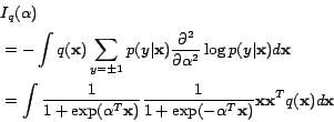
Let
be the objective function in
(15). We then have
Using the convexity property of reciprocal function, namely
 for and pdf
 , we can arrive at the following
deduction:
, we can arrive at the following
deduction:
Substituting the above inequation back into (19), we
can achieve the following inequality:
This finishes the proof of the inequality mentioned above.