In this paper, we present a detailed study of the following problem: given a small but cohesive "seed set" of web pages, expand this set to generate the enclosing community (or communities). This seed expansion problem has been addressed by numerous researchers as an intermediate step of various graph-based analyses on the web. To our knowledge, however, it has never been called out as an interesting primitive in its own right. As we will show, the mathematical structure underlying the problem is rich and fruitful, and allows us to develop algorithms that perform dramatically better than naive approaches.
The seed expansion problem first came into prominence in 2000, when Jon Kleinberg introduced the HITS algorithm [7]. That algorithm used a search engine to generate a seed set, and then performed a fixed-depth neighborhood expansion in order to generate a larger set of pages upon which the HITS algorithm was employed. This general recipe has since seen broad adoption, and is now a common technique for local link-based analysis. Variants of this technique have been employed in community finding [8], in finding similar pages [1], in variants of HITS, PageRank [13], and TrustRank [5], and in classification [2]. More sophisticated expansions have been applied by Flake et al. [4] in the context of community discovery.
Alongside this body of work in web analysis, the theoretical computer science community has developed algorithms that find cuts of provably small conductance within a carefully expanded neighborhood of a vertex [12]. Intuitively, these methods are efficient because they make non-uniform expansion decisions based on the structure revealed during exploration of the neighborhood surrounding the vertex. Our results are based on these techniques, and we present modified versions of these methods and theorems that apply to the seed set expansion problem.
The actual computation is done by simulating a ``truncated'' random walk for a small number of steps, starting from a distribution concentrated on the seed set. In each step of the truncated walk, probability is spread as usual to neighboring vertices, but is then removed from any vertex with probability below a certain threshold. This bounds the number of vertices with nonzero probability, and implicitly determines which vertices are examined. After each step in the expansion process, we examine a small number of sets determined by the current random walk distribution, and eventually choose one of these sets to be the community for the seed.
The graphs we consider in our experiments have small diameter and a small average distance between nodes, so the number of nodes within a fixed distance of the seed set grows quickly. Nonetheless, these graphs contain distinct communities with relatively small cutsizes. We assume that the seed set is largely contained in such a community, which we refer to as a target community. In many of the graphs we consider, the seed is contained in a nested sequence of target communities. The results in section 2.5 show that if a good target community exists for the seed, then the random walk method produces some community that is largely contained within this target.
When expanding the seed with a truncated walk, a target community serves as a bottleneck, containing much of the probability for a significant number of steps. Since probability is removed from low-probability vertices, this prevents the support of the walk from expanding quickly beyond the bottleneck. In contrast, expanding the seed set using a fixed-depth expansion entirely ignores the bottleneck defining the community. Some branch of the BFS tree is likely to cross the bottleneck and rapidly expand in the main graph before a large fraction of the nodes in the community have been reached. Thus a fixed depth expansion will be a bad approximation to the community, and might also be an impractically large ``candidate set'' for further processing.
The goal of examining a small number of nodes is clear enough, but we also need to pin down what we mean by a ``good'' community containing a given seed set. We will do this by describing the limitations of several possible ways to define good communities.
Several papers including [4] have defined a community to be a subgraph bounded by a small cut, which can be obtained by first growing a candidate set using BFS, and then pruning it back using ST max-flow. Unfortunately, a small seed set will often be bounded by a cut that is smaller than the cut bounding the target community, so the mininum cut criterion will not want to grow the seed set. Flake et al. address this problem by performing this process several times, adding nodes from the candidate set at each step to ensure expansion.
Another idea for ensuring a reasonable expansion of the seed set that is less ad hoc than most is to optimize for conductance instead of cutsize alone. Graph conductance (aka the normalized cut metric) is a quotient-style metric that provides an incentive for growing the seed set. Unfortunately, the conductance score can be improved by adding barely related nodes (or even a disconnected component) to the seed set. We need to ensure that only nearby nodes are added to the seed set.
This raises a subtle but important point. While stronger parametric flow methods do exist for finding low-conductance cuts within an expanded neighborhood of the seed set, our walk-based method's weaker spectral-style guarantee on conductance is counterbalanced by a valuable ``locality'' property which ensures that we output a community consisting of nodes that are closely related to the seed set. In practice we try to get the best of both worlds by cleaning up the walk-based cuts with a conservative use of flow that does not disturb this locality property very much. Experiments show that the results compare well with stronger optimization techniques.
The random walks techniques are remarkable because they produce communities with conductance guarantees, yet can be computed locally rather than on the whole graph, often while touching fewer nodes than BFS would. The best low-conductance cuts are more likely than minimum cuts to non-trivially expand the seed set, but still ensure a small boundary defining a natural community. Finally, in a certain sense that we will discuss in section 2.5, the added nodes are close to the seed set.
As part of their work on graph partitioning and graph sparsification [12], Spielman and Teng present a method for finding cuts based on the mixing of a random walk starting from a single vertex. In that paper, the method is used as a subroutine to produce balanced separators and multiway partitions.
In this section, we describe how to use the techniques developed by Spieman-Teng to find communities from a seed set, and describe how the size and quality of the seed set affects the results. In sections 2.1-2.3 we present background on random walks and sweeps. In section 2.4 we show that any seed set that makes up a significant fraction of a target community will produce good results with our seed expansion method, and that most seed sets that are chosen randomly from within a target community will also produce good results. In section 2.5 we present a stripped-down version of the local partitioning techniques developed by Spielman-Teng, and describe quantitatively how the size and quality of the seed set affect the running time and guarantees. In section 2.6 we describe the truncation method used by Spielman-Teng, and describe the heuristics and practical modifications we have employed to keep the running time and total number of vertices examined small.
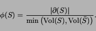
This definition of conductance should not be confused with the conductance associated with a particular random walk on the graph. In particular, the conductance associated with a lazy random walk is a factor of 2 smaller.
![\begin{displaymath}H_{t}(k) = \left [ P_{t}(k) - \frac{k}{2m} \right ].\end{displaymath}](p3095-andersen-img46.png)
![\begin{displaymath}\vert p_t - \psi_{V} \vert = 2 \max_{A \subseteq V} \langle... ...{V},1_{A} \rangle = 2 \max_{k} \left [ H_{t}(k) \right ] .\end{displaymath}](p3095-andersen-img54.png)
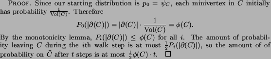
Any set that is fairly large and nearly contained in the target community is also a good seed set. The bounds in the lemma below are weak for smaller seed sets, but are sufficient for seed sets that make up a significant fraction of the target community.
Seed sets chosen randomly from within a target community are also likely to be good seed sets for that community. The following result is stated without proof, since it follows by applying a Chernoff-type bound to a weighted sum of independent random variables in the usual way.
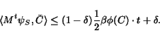
The following is a stripped-down version of a theorem of Spielman-Teng, extended for a seed set instead of a single starting vertex.

The sweep cut ![]() can be viewed as a community of the seed
can be viewed as a community of the seed
![]() . In addition to
having small conductance, there is a significant drop in
probability outside
. In addition to
having small conductance, there is a significant drop in
probability outside ![]() by Theorem 1. Figure 3 shows an example
of this simultaneous small conductance cut and probability
drop.
by Theorem 1. Figure 3 shows an example
of this simultaneous small conductance cut and probability
drop.
While these guarantees on ![]() are fairly clear, the way that the
community is related to the seed set is more subtle. The most
obvious thing we can say about this relationship is probably
the most important: the community is obtained by taking all
vertices where the value of
are fairly clear, the way that the
community is related to the seed set is more subtle. The most
obvious thing we can say about this relationship is probably
the most important: the community is obtained by taking all
vertices where the value of
![]() is above a certain
threshold. If we view
is above a certain
threshold. If we view ![]() as a measure of closeness to the seed
set, this is a strong guarantee.
as a measure of closeness to the seed
set, this is a strong guarantee.
Unfortunately, ![]() is not a good measure of closeness to
the seed set when
is not a good measure of closeness to
the seed set when ![]() becomes large. As
becomes large. As ![]() tends
to infinity,
tends
to infinity, ![]() tends to a constant, and the ordering of
the vertices determined by
tends to a constant, and the ordering of
the vertices determined by ![]() tends to the same ordering determined by
the second-largest eigenvector of
tends to the same ordering determined by
the second-largest eigenvector of ![]() , which is independent of the seed set if
the graph is connected. This means that the vertices from the
seed set are not guaranteed to have the largest values of
, which is independent of the seed set if
the graph is connected. This means that the vertices from the
seed set are not guaranteed to have the largest values of
![]() , and so
the seed set is not necessarily contained in the resulting
community. However, we have an upper bound on the number of
walk steps taken, and we claim that
, and so
the seed set is not necessarily contained in the resulting
community. However, we have an upper bound on the number of
walk steps taken, and we claim that ![]() is a good
measure of relationship to the seed set for small values of
is a good
measure of relationship to the seed set for small values of
![]() . In practice, we
have observed that requiring the community to be determined
by a threshold on the values of
. In practice, we
have observed that requiring the community to be determined
by a threshold on the values of ![]() rules out more degenerate behavior than
requiring only that the community contains the seed.
rules out more degenerate behavior than
requiring only that the community contains the seed.
We cannot hope that the resulting community ![]() will
closely match the target community
will
closely match the target community ![]() , without
placing additional assumptions on the communities inside
, without
placing additional assumptions on the communities inside ![]() . Instead, the
target community is used to ensure that some community for
. Instead, the
target community is used to ensure that some community for
![]() will be found,
and this community is likely to be mostly contained within
the target community. This can be made precise if a stronger
restriction is placed on
will be found,
and this community is likely to be mostly contained within
the target community. This can be made precise if a stronger
restriction is placed on ![]() . Spielman-Teng showed that if
. Spielman-Teng showed that if ![]() is roughly
is roughly
![]() , then the
gap in probability described in Theorem 1 can be used to
show that the majority of vertices in
, then the
gap in probability described in Theorem 1 can be used to
show that the majority of vertices in ![]() are
contained in
are
contained in ![]() .
.
The actual subroutine created by Spielman-Teng, called Nibble, has a stronger guarantee than the method we have presented here. One aspect of Nibble that we would like to reproduce is the ability to find a small community near the seed set while keeping the number of vertices examined small. This is accomplished by using truncated walk distributions in place of exact walk distributions.
In the truncated walk, the probability on any vertex where
![]() is set to 0 after each
step. This ensures that the support of the truncated walk
is set to 0 after each
step. This ensures that the support of the truncated walk
![]() is small,
which gives a bound on the running time of the algorithm,
since the time required to perform a step of the random walk
and a sweep depends on
is small,
which gives a bound on the running time of the algorithm,
since the time required to perform a step of the random walk
and a sweep depends on
![]() . For the theoretical
guarantees to apply, the truncation parameter
. For the theoretical
guarantees to apply, the truncation parameter ![]() must be
small enough so that
must be
small enough so that ![]() is smaller than the probability gap
is smaller than the probability gap
![]() implied by Theorem 1.
implied by Theorem 1.
In our experiments we perform a more severe kind of
truncation, at a stronger level than is supported by these
guarantees. We specify a target volume ![]() , sort the
vertices in terms of
, sort the
vertices in terms of ![]() for the current truncated
probability vector
for the current truncated
probability vector ![]() ,
and let
,
and let ![]() be the last
index such that
be the last
index such that
![]() . We then remove the probability from all vertices
. We then remove the probability from all vertices ![]() where
where
![]() . In
section 3.6 we will
experimentally show that a target cluster can be accurately
found by setting
. In
section 3.6 we will
experimentally show that a target cluster can be accurately
found by setting ![]() somewhat larger than the cluster size.
somewhat larger than the cluster size.
|
The previous sections contained theorems proving that given a sufficiently distinct target set (a subgraph with small enough conductance) and a sufficiently ``good'' seed set lying mostly within it, a lazy local random walk will grow the seed set and return a low-conductance community for the seed set. We also proved that good seed sets are not rare, and that a big enough or random subset of the target set should be good.
Due to constant factors, it is often hard to tell whether a theoretical method will work in practice. Therefore in the following subsections we will describe sanity check experiments on three datasets in which we used a sparse matrix viewer to choose target sets and seed sets that appeared likely to satisfy the preconditions of the theorems, so that we could check whether the method actually recovered the target sets with reasonable accuracy.
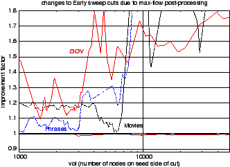
There are several reasons for using flow to clean up the sweep cuts. First, it is generally a good idea to do this for any spectral-type graph partitioning method [9]. Second, aggressive probability truncation can produce cuts that are even noisier than usual. Third, in the following sections we will see empirical evidence that flow-based improvement makes the sweep cut method less sensitive to the number of walk steps that are taken.
However, this post-processing needs to be done with care; in some preliminary experiments in which we grew well past the size of the target set and then used parametric flow to shrink back to the cut with optimal conductance of any cut containing the seed set, we sometimes got surprising solutions containing distant, essentially unrelated nodes. Those results were a clear demonstration that conductance and containment of the seed set do not entirely capture our goals in seed set expansion. We actually want to find a low-conductance set that is obtained by adding nearby nodes to the seed set. Back in section 2.5 we argued that if a set of nodes contains a lot of probability from a random walk that hasn't run for too many steps, then it has a version of the desired locality property.
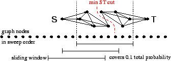
To improve the sweep cuts without sacrificing the locality property, we did some conservative post-processing with repeated ST max flow calculations across a sliding window covering 10 percent of the total probability.1 These calculations were free to rearrange the lower probability nodes near a bottleneck, but not the higher probability nodes near the seed set, thus allowing us to reduce the cutsize without risking the loss of too much enclosed probability. The plots in Figure 1 show that our actual losses of enclosed probability were typically at least an order of magnitude smaller than the cutsize improvement factors.
|
|
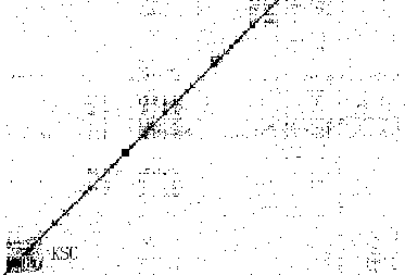
The starting point for this graph was TREC's well-known .GOV web dataset. To make the graph's block structure more obvious (so that we could visually choose a seed set that probably satisfies the requirements of the theory), we repeatedly deleted all nodes with in- or out-degree above 300 or equal to 1 or 2. Then we symmetrized the graph and extracted the largest connected component, yielding an undirected graph with 536560 nodes and 4412473 edges, and node degrees ranging from 3 to 394.
After inspecting this graph's adjacency matrix (see Figure 2), we chose for our target cluster a distinct matrix block containing roughly 3000 URL's associated with the Kennedy Space Center. Among these URL's were 830 beginning with science.ksc.nasa.gov/shuttle. We randomly selected 230 of these nodes as a seed set. Jumping ahead to our results, Table 1 shows that by growing this seed set we can recover nearly all of the science.ksc.nasa.gov/shuttle URL's, plus large fractions of several other families of URL's that relate to the Kennedy Space Center.
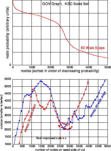
Figure 3-top shows the probability distribution after 60 steps of a lazy random walk starting with uniform probability on the seed set and zero probability elsewhere. Along the x axis nodes are sorted in order of decreasing degree-normalized probability, which we call ``sweep order''. On the left are the high probability nodes that are close to the seed set. Lower probability nodes appear towards the right of the plot and beyond. The sharp decrease in probability around 2500-3000 nodes is the signature of the low-conductance bottleneck that we are interpreting as a cluster boundary.
Each curve in Figure 3-bottom shows a ``cutsize sweep'' in which we evaluate all cuts between adjacent nodes in the sweep order defined by the probability distribution at some step in the local random walk.2 The two curves here are for 30 and 90 steps. Notice that both sweeps show a dip in cutsize around 2500-3000 nodes, which again reveals the bottleneck at the cluster boundary.
Comparing the 30- and 90-step sweeps, we see that the 30-step sweep looks better towards the left, while the 90-step sweep looks better towards the right. This is because the spreading probability is revealing information about larger sets later. We also see that the flow-improved solutions for 30 and 90 steps are nearly the same; apparently the flow-based post-processing helps us get good results for a wider range of stopping times.This task illustrates what can happen when cluster nesting causes there to be more than one reasonable community for the seed set. The data originated in Yahoo's ``sponsored search'' business (Google's ``ad words'' is roughly similar). In this business advertisers make bids on (bidded phrase, advertiser URL) pairs, which can be encoded in a bipartite graph with bidded phrases on one side and advertiser URL's on the other, with each bid represented by an edge. Co-clustering this graph reveals block structure showing that the overall advertising market breaks down into numerous submarkets associated with flowers, travel, financial services, etc. For our experiment we used a 2.4 million node, 6 million edge bipartite graph built from part of an old version of the sponsored search bid database. Node degrees ranged from 1 to about 30 thousand.
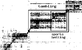
Based on earlier experiences we expected that this dataset would contain a distinct gambling cluster which would contain a subcluster focused on sports betting (see the matrix picture in Figure 4). For a seed set we used grep to find all bidded phrases and advertiser URL's containing the substring ``betting''. This resulted in a 594-node seed set which includes nodes on both sides of the bipartite graph, and is probably mostly contained within the sports betting subcluster.
Our seed set lies within the sports betting cluster, and this in turn lies within the gambling cluster. To which of these clusters should the seed set be expanded? Perhaps the algorithm should tell us about both of the possible answers. In fact, when there are nested clusters surrounding a seed set, over time the local random walk method often does tell us about more than one possible answer as the probability distribution spreads out.
|
|
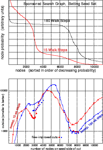
This behavior can be very clearly seen in the probability distributions plotted in Figure 5-top. At 15 steps there is a sharp decrease in probability marking the boundary of the 3000-node betting subcluster. At 180 steps there is a different sharp decrease in probability marking the boundary of the enclosing 8000-node gambling cluster. Notice that within this larger cluster the probabilities are becoming quite uniform at 180 steps, so it is no longer easy to see the boundary of the inner cluster.
The cutsize sweeps of Figure 5-bottom show what all this means in terms of cuts. At 15 steps the boundary of the inner cluster is sharply defined by a dip in cutsize near 3000 nodes. Also at this point we are starting to get a rough preview of the boundary of the enclosing cluster. This preview is much improved by the flow-based post-processing.
At 180 steps, the inner dip in cutsize delimiting the betting subcluster has been washed out (but can be somewhat recovered with flow) but now we have a good dip near 8000 nodes which is the boundary of the outer gambling cluster.
|
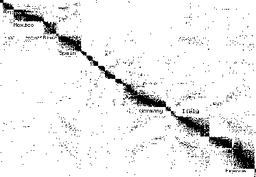
This task has even more cluster nesting than the previous one. The graph is bipartite and was built from the IMDB file relating movies and actresses. It has a clear block structure that is strongly correlated with countries.3 Therefore we use country-of-production labels for the movies as cluster membership labels for purposes of choosing seed sets and measuring precision and recall.
We cleaned up the problem a bit by deleting all multi-country movies and many non-movie items such as television shows and videos. We combined several nearly synonymous country labels (e.g. USSR and Russia) and then deleted all but the top 30 countries. Finally we deleted all degree-1 nodes and extracted the largest connected component. We ended up with a bipartite graph with 77287 actress nodes, 121143 movie nodes, and 566756 edges. The minimum degree was 2, and the maximum degree was 690.
For a target cluster we chose Spain, whose matrix block can be seen in Figure 10. It appears to part of a super-cluster containing other Spanish- and Portuguese-language countries. One can also see many cross edges denoting appearances of Spanish actresses in French and Italian movies, and vice versa, so a Romance-language supercluster would not be surprising. For a seed set we randomly selected 5 percent of the movies produced in Spain. This seed set contained 179 movie nodes, and 0 actress nodes.
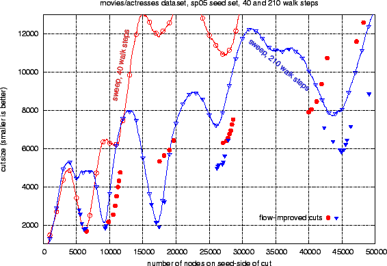
The curves in Figure 6 show cutsize sweeps based on the probability distribution after 40 and 210 walk steps. The 40-step sweep (open circles) contains a sharp dip at 6500 nodes which marks the boundary of the Spain cluster with high accuracy. Beyond this bottleneck the 40-step sweep is pretty sketchy, but the flow-based cuts derived from it (filled circles) are already surprisingly good.
The open triangle curve in Figure 6 shows that at 210 steps, the random walk has already washed out the boundary of the Spain cluster, but is now giving a better view of the enclosing hierarchy of four superclusters, especially those containing 9000 and 17500 nodes. The filled triangles show that flow-based post-processing recovers the washed-out boundary of the Spain cluster, and greatly improves the boundaries of the 27000 and 45000 node superclusters.
Because we have country labels for the movies we can interpret these clusters, and also measure the accuracy with which they are being recovered. The following table contains precision and recall measurements for the movies4 in the sets of nodes delimited by the (flow-improved) leftmost, middle, and rightmost dips in Figure 6. These precision and recall measurements show that the 6500-node set is a good approximation of our target cluster of Spain. The 17500-node set (which has the smallest conductance) is a very good approximation of a mostly Spanish-language supercluster containing Spain, Mexico, and Argentina, plus Portugal. The 45000-node set is a good approximation of a Romance-language supercluster containing the previous 4 countries plus Brazil, Italy, and France.
| quotient = cutsize / nodes | preci. | recall | cluster contents |
| 0.255835 = 1666 / 6512 | 0.956 | 0.979 | Spain |
| 0.109531 = 1910 / 17438 | 0.979 | 0.995 | Spanish+Portugal |
| 0.129574 = 5821 / 44924 | 0.958 | 0.988 | Romance language |
|
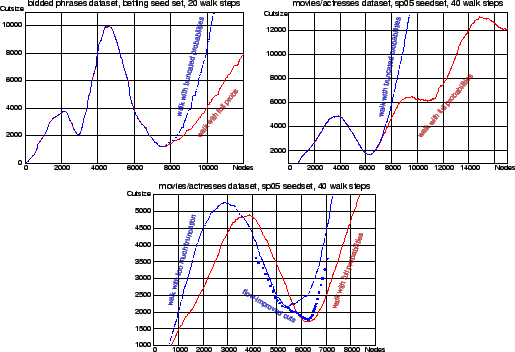
In the experiments up to now we have done full walks with probability spreading to the whole graph. The computation can be made more local by doing a truncated walk, as discussed in section 2.6. Here we briefly examine the qualititative effect of truncating to a fixed number of nodes after each step. Figure 7 compares cut sweeps over node orderings derived from truncated and untruncated walks on the sponsored search and movies/actresses graphs. In the first two plots we truncated to the top 10000 nodes after each step. Up through the bottlenecks near 8000 and 6500 nodes, respectively, these new sweeps look similar to the earlier sweeps over full walks. In the final plot we truncated to 6000 nodes on the movies/actresses task, which is a bit too small for recovering the 6500-node Spain cluster. In this case the results are degraded, but somewhat recoverable with flow-based post-processing.
|
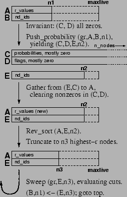
One of the main features of the truncated random walks
partitioning method is that its time and space requirements
can be independent of the graph size. We will describe some
code that basically achieves this time independence.
[However, it still uses ![]() working space.] Our data structures, and the
algorithm for one iteration are sketched in Figure 8. The graph
contains
working space.] Our data structures, and the
algorithm for one iteration are sketched in Figure 8. The graph
contains ![]() nodes
and
nodes
and ![]() edges, and is
representable in CSR format in (n+1)*4 + 2*m*4 bytes.
edges, and is
representable in CSR format in (n+1)*4 + 2*m*4 bytes.
We use five working arrays. ![]() is a scratch array for probabilities containing
is a scratch array for probabilities containing
![]() doubles, mostly
zero.
doubles, mostly
zero. ![]() is a scratch array
containing
is a scratch array
containing ![]() flag
bytes, mostly zero. Together they occupy
flag
bytes, mostly zero. Together they occupy ![]() bytes.5 We use parallel arrays of
doubles and node_id's to compactly represent small sets of
nonzero values associated with ``active'' nodes. ``Maxlive''
is an upper bound on the number of active nodes.
bytes.5 We use parallel arrays of
doubles and node_id's to compactly represent small sets of
nonzero values associated with ``active'' nodes. ``Maxlive''
is an upper bound on the number of active nodes. ![]() and
and ![]() are two arrays
of node_id's each consuming
are two arrays
of node_id's each consuming
![]() bytes.
bytes. ![]() is an array of
is an array of
![]() -values
(degree-normalized probabilities) consuming
-values
(degree-normalized probabilities) consuming
![]() bytes.
bytes.
The key to speed and scalability is to never do any ![]() -time
operation, including clearing arrays
-time
operation, including clearing arrays ![]() or
or ![]() , except at program
initialization time. While expanding a seed set, we only do
operations whose time depends on the number of active nodes.
, except at program
initialization time. While expanding a seed set, we only do
operations whose time depends on the number of active nodes.
Push_probability
![]() works as follows. The input
works as follows. The input ![]() represents the
represents the ![]() currently
active nodes. We zero the counter
currently
active nodes. We zero the counter ![]() . The arrays
. The arrays ![]() and
and ![]() are
already zeroed. For each active node we push half of its
probability to itself, while the other half is evenly divided
and pushed to its neighbors. To push some probability
are
already zeroed. For each active node we push half of its
probability to itself, while the other half is evenly divided
and pushed to its neighbors. To push some probability ![]() to node
to node ![]() , we do:
, we do:
{
![]() +
+![]() ; if (0=
; if (0=![]() ) {
) {
![]() +
+![]() }}.
We end up with
}}.
We end up with ![]() nonzero probabilities scattered in
nonzero probabilities scattered in ![]() . The
. The ![]() entries in
entries in
![]() tell where they
are, so we can gather them back into
tell where they
are, so we can gather them back into ![]() , simultaneously
clearing the nonzeros in
, simultaneously
clearing the nonzeros in ![]() and
and ![]() .
.
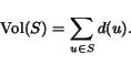
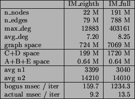
We now describe some timings on two large graphs. The
191-million node graph IM_full is a symmetrized version of
the buddy list graph for users of Yahoo Instant Messenger. We
used an out-of-core reimplementation of Metis to partition
this graph into 8 big pieces, one of which is the 22-million
node graph IM_eighth. We also used Metis [6] to break both
graphs into numerous tiny pieces of size 150-200. For each
graph, we randomly selected 100 of these tiny pieces to serve
as seed sets for 100 runs of our truncated random walk
procedure. Each run went for 100 iterations. We used
volume-based truncation, on each step cutting back to a
volume (sum of degrees) of 20000. On average, the probability
pushing step grew the active set from about ![]() nodes out
to about
nodes out
to about ![]() nodes, then the truncation step cut it
back to about
nodes, then the truncation step cut it
back to about ![]() nodes.
nodes.
Figure 9
summarizes these graphs and runs, which were done on a
4-processor 2.4 GHz Opteron with 64 Gbytes of RAM. The
average time per iteration was only 9.2 and 13.5 msec for the
two graphs. Iterations on IM_full took 1.5 times longer, even
though the graph is 8 times bigger. We actually hoped that
the iteration time would be the same. A possible explanation
for the increase is that there were more cache misses for the
bigger graph (the probability pushing step involves a pattern
of ``random'' memory accesses). To put these times into
perspective, we also list some ``bogus'' times where we
actually checked our invariant that the C and D arrays are
zeroed at the top of the loop. This checking takes ![]() time,
resulting in a huge increase in time per step, and a factor
of 8 increase from the smaller to larger graph.
time,
resulting in a huge increase in time per step, and a factor
of 8 increase from the smaller to larger graph.
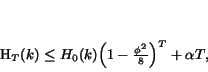
So far we haven't said much about how to choose values for
the parameters ![]() (the
number of walk steps), and
(the
number of walk steps), and ![]() (the truncation size). It is clear from the
previous sections that a seed set can have several possible
communities; to choose between them we would need to retain
some freedom in choosing parameter values. According to
Theorem 1,
it suffices to set
(the truncation size). It is clear from the
previous sections that a seed set can have several possible
communities; to choose between them we would need to retain
some freedom in choosing parameter values. According to
Theorem 1,
it suffices to set ![]() to be
roughly
to be
roughly
![]() , where
, where ![]() is a lower
bound on the desired conductance and
is a lower
bound on the desired conductance and ![]() is an upper
bound on the expansion factor
is an upper
bound on the expansion factor
![]() . [We note that
the method often works with much smaller values for
. [We note that
the method often works with much smaller values for ![]() .]
.]
One can obtain an algorithm that depends on a single
parameter by choosing a value of ![]() and searching through several values of
and searching through several values of ![]() , setting
, setting
![]() , and
, and
![]() . The table below shows
the results of such a search on the movies/actresses task,
with
. The table below shows
the results of such a search on the movies/actresses task,
with ![]() set to
set to ![]() , and with
, and with ![]() set to
set to ![]() for each
for each
![]() between 5 and 10.
For each value of
between 5 and 10.
For each value of ![]() , we
return the cut with the smallest conductance found by any of
the
, we
return the cut with the smallest conductance found by any of
the ![]() sweeps. The
following table reports the conductance and volume of this
cut, and also the step
sweeps. The
following table reports the conductance and volume of this
cut, and also the step ![]() at which it was found.
at which it was found.
|
|
|
|
conductance | volume | t |
|
|
|
|
.1280 | 27621 | 480 |
|
|
|
|
.0452 | 37499 | 250 |
|
|
|
|
.0240 | 103720 | 700 |
|
|
|
|
.0193 | 103894 | 280 |
|
|
|
|
.0162 | 127374 | 620 |
|
|
|
|
.0129 | 835500 | 780 |
|