| Soumen Chakrabarti | Kriti Puniyani | Sujatha Das | ||
| IIT Bombay | IIT Bombay | IIT Bombay | ||
| Corpus/index | Size (GB) |
| Original corpus | 5.72 |
| Gzipped corpus | 1.33 |
| Stem index | 0.91 |
| Full atype index | 4.30 |
| Reachability index | 0.005 |
| Forward index | 1.16 |
|
|
| (3) |
| (4) |
| (5) |
| b from | Train | Test | R300 | MRR |
| IR-IDF | - | 2000 | 211 | 0.16 |
| RankExp | 1999 | 2000 | 231 | 0.27 |
| RankExp | 2000 | 2000 | 235 | 0.31 |
| RankExp | 2001 | 2000 | 235 | 0.29 |
| 100 | integer#n#1 |
| 78 | location#n#1 |
| 77 | person#n#1 |
| 20 | city#n#1 |
| 10 | name#n#1 |
| 7 | author#n#1 |
| 7 | company#n#1 |
| 6 | actor#n#1 |
| 6 | date#n#1 |
| 6 | number#n#1 |
| 6 | state#n#2 |
| 5 | monarch#n#1 |
| 5 | movie#n#1 |
| 5 | president#n#2 |
| 5 | inventor#n#1 |
| 4 | astronaut#n#1 |
| 4 | creator#n#2 |
| 4 | food#n#1 |
| 4 | mountain#n#1 |
| 4 | musical_instrument#n#1 |
| 4 | newspaper#n#1 |
| 4 | sweetener#n#1 |
| 4 | time_period#n#1 |
| 4 | word#n#1 |
| 3 | state#n#1 |
| 3 | university#n#1 |
|
|
| (7) |
|
|
|
|
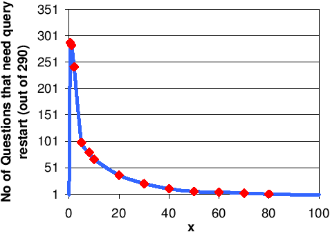
| Ratio £ | Count | % | Ratio £ | Count | % |
| .5-1 | 16 | 11.6 | 10-20 | 110 | 79.7 |
| 1-2 | 78 | 56.5 | 20-50 | 123 | 89.1 |
| 2-5 | 93 | 67.3 | 50-100 | 128 | 92.8 |
| 6-10 | 104 | 75.3 | 100-200 | 138 | 100 |
|
|