Random Sampling from a Search Engine's Index
1 Introduction
The latest round in the search engine size wars (cf. [22]) erupted last August after Yahoo! claimed [20] to index more than 20 billion documents. At the same time Google reported only 8 billion pages in its index, but simultaneously announced [3] that its index is three times larger than its competition's. This surreal debate underscores the lack of widely acceptable benchmarks for search engines.
Current evaluation methods for search engines [11,14,6] are labor-intensive and are based on anecdotal sets of queries or on fixed TREC data sets. Such methods do not provide statistical guarantees about their results. Furthermore, when the query test set is known in advance, search engines can manually adapt their results to guarantee success in the benchmark.
In an attempt to come up with reliable automatic benchmarks for search engines, Bharat and Broder [4] proposed the following problem: can we sample random documents from a search engine's index using only the engine's public interface? Unlike the manual methods, random sampling offers statistical guarantees about its test results. It is important that the sampling is done only via the public interface, and not by asking the search engine itself to collect the sample documents, because we would like the tests to be objective and not to rely on the goodwill of search engines. Furthermore, search engines seem reluctant to allow random sampling from their index, because they do not want third parties to dig into their data.
Random sampling can be used to test the quality of search engines under a multitude of criteria: (1) Overlap and relative sizes: we can find out, e.g., what fraction of the documents indexed by Yahoo! are also indexed by Google and vice versa. Such size comparisons can indicate which search engines have better recall for narrow-topic queries. (2) Topical bias: we can identify themes or topics that are overrepresented or underrepresented in the index. (3) Freshness evaluation: we can evaluate the freshness of the index, by estimating the fraction of ``dead links'' it contains. (4) Spam evaluation: using a spam classifier, we can find the fraction of spam pages in the index. (5) Security evaluation: using an anti-virus software, we can estimate the fraction of indexed documents that are contaminated by viruses.
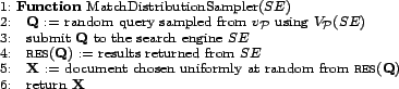
The Bharat-Broder approach. Bharat and Broder proposed
the following simple algorithm for uniformly sampling documents
from a search engine's index. The algorithm successively
formulates ``random'' queries, submits the queries to the search
engine, and picks uniformly chosen documents from the result sets
returned. In order to construct the random queries, uses a
lexicon of terms that appear in web documents. Each term
in the lexicon should be accompanied by an estimate of its
frequency on the web. Random queries are then formulated as
conjunctions or disjunctions of terms that are randomly selected
from the lexicon, based on their estimated frequency. The lexicon
is constructed at a pre-processing step by crawling a large
corpus of documents (Bharat and Broder crawled the Yahoo!
directory).
As Bharat and Broder noted in the original article [4] and was later observed by
subsequent studies [7],
the method suffers from severe biases. The first bias is towards
long, ``content-rich'', documents, simply because these documents
match many more queries than short documents. An extreme example
is online dictionaries and word lists (such as the ispell
dictionaries), which will be returned as the result of almost any
query. Worse than that, when queries are formulated as
conjunctions or disjunctions of unrelated terms, typically
only dictionaries and word lists match the queries.
Another major problem is that search engines do not allow access
to the full list of results, but rather only to the top
![]() ones (where
ones (where ![]() is usually 1,000). Since
the Bharat-Broder technique samples documents only from the top
is usually 1,000). Since
the Bharat-Broder technique samples documents only from the top
![]() , it is biased towards
documents that have high static rank. Finally, the accuracy of
the Bharat-Broder method is directly related to the quality of
the term frequency estimates it uses. In particular, if these
estimates are biased, then the same bias will be reflected in the
samples. Collecting accurate term statistics is a major problem
by itself, and it is not clear that using a web directory like
Yahoo! is sufficient.
, it is biased towards
documents that have high static rank. Finally, the accuracy of
the Bharat-Broder method is directly related to the quality of
the term frequency estimates it uses. In particular, if these
estimates are biased, then the same bias will be reflected in the
samples. Collecting accurate term statistics is a major problem
by itself, and it is not clear that using a web directory like
Yahoo! is sufficient.
Our contributions. We propose two novel methods for
sampling pages from a search engine's index. Our first technique
uses a lexicon to formulate random queries, but unlike the
Bharat-Broder approach, does not need to know term frequencies.
Our second technique is based on a random walk on a virtual graph
defined over the documents in the index. This technique does not
need a lexicon at all.
Both our techniques, like the Bharat-Broder method, produce
biased samples. That is, some documents are more likely
to be sampled than others. Yet, our algorithms have one crucial
advantage: they produce together with each sample document
![]() a corresponding
``weight''
a corresponding
``weight''
![]() , which
represents the probability
, which
represents the probability
![]() of the
document to be sampled. This seemingly minor difference turns out
to be extremely significant. The weights allow us to apply
stochastic simulation methods on the samples and
consequently obtain uniform, unbiased, samples from the
search engine's index!
of the
document to be sampled. This seemingly minor difference turns out
to be extremely significant. The weights allow us to apply
stochastic simulation methods on the samples and
consequently obtain uniform, unbiased, samples from the
search engine's index!
A simulation method accepts samples taken from a trial
distribution ![]() and
simulates sampling from a target distribution
and
simulates sampling from a target distribution
![]() . In order for the
simulation to be feasible, the simulator needs to be able to
compute
. In order for the
simulation to be feasible, the simulator needs to be able to
compute
![]() and
and
![]() , at least
up to normalization, given any instance
, at least
up to normalization, given any instance
![]() . The simulation
has some overhead, which depends on how far
. The simulation
has some overhead, which depends on how far ![]() and
and ![]() are from each other. In
our case
are from each other. In
our case ![]() is the uniform
distribution over the search engine's index, and
is the uniform
distribution over the search engine's index, and ![]() is the distribution of
samples generated by our samplers. We employ three Monte Carlo
simulation methods: rejection sampling, importance
sampling, and the Metropolis-Hastings
algorithm.
is the distribution of
samples generated by our samplers. We employ three Monte Carlo
simulation methods: rejection sampling, importance
sampling, and the Metropolis-Hastings
algorithm.
One technical difficulty in applying simulation methods in our
setting is that the weights produced by our samplers are only
approximate. To the best of our knowledge, stochastic
simulation with approximate weights has not been addressed
before. We are able to show that the rejection sampling method
still works even when provided with approximate weights. The
distribution of the samples it generates is no longer identical
to the target distribution ![]() , but is rather only close to
, but is rather only close to ![]() . Similar analysis for importance sampling and for the
Metropolis-Hastings algorithm is deferred to future work, but our
empirical results suggest that they too are affected only
marginally by the approximate weights.
. Similar analysis for importance sampling and for the
Metropolis-Hastings algorithm is deferred to future work, but our
empirical results suggest that they too are affected only
marginally by the approximate weights.
Pool-based sampler. A query pool is a
collection of queries. Our pool-based sampler assumes knowledge
of some query pool ![]() .
The terms constituting queries in the pool can be collected by
crawling a large corpus, like the Yahoo! or ODP [9] directories. We stress again
that knowledge of the frequencies of these terms is not
needed.
.
The terms constituting queries in the pool can be collected by
crawling a large corpus, like the Yahoo! or ODP [9] directories. We stress again
that knowledge of the frequencies of these terms is not
needed.
The volume of a query
![]() is the number of
documents indexed by the search engine and that match
is the number of
documents indexed by the search engine and that match
![]() . We first show
that if the sampler could somehow sample queries from the pool
proportionally to their volume, then we could attach to each
sample a weight. Then, by applying any of the simulation methods
(say, rejection sampling), we would obtain truly uniform samples
from the search engine's index. Sampling queries according to
their volume is tricky, though, because we do not know a priori
the volume of queries. What we do instead is sample queries from
the pool according to some other, arbitrary, distribution (e.g.,
the uniform one) and then simulate sampling from the
volume distribution. To this end, we use stochastic simulation
again. Hence, stochastic simulation is used twice: first to
generate the random queries and then to generate the uniform
documents.
. We first show
that if the sampler could somehow sample queries from the pool
proportionally to their volume, then we could attach to each
sample a weight. Then, by applying any of the simulation methods
(say, rejection sampling), we would obtain truly uniform samples
from the search engine's index. Sampling queries according to
their volume is tricky, though, because we do not know a priori
the volume of queries. What we do instead is sample queries from
the pool according to some other, arbitrary, distribution (e.g.,
the uniform one) and then simulate sampling from the
volume distribution. To this end, we use stochastic simulation
again. Hence, stochastic simulation is used twice: first to
generate the random queries and then to generate the uniform
documents.
We rigorously analyze the pool-based sampler and identify the properties of the query pool that make this technique accurate and efficient. We find that using a pool of phrase queries is much more preferable to using conjunctive or disjunctive queries, like the ones used by Bharat and Broder.
Random walk sampler. We propose a completely different
sampler, which does not use a term lexicon at all. This sampler
performs a random walk on a virtual graph defined over the
documents in the index. The limit equilibrium distribution of
this random walk is the uniform distribution over the documents,
and thus if we run the random walk for sufficiently many steps,
we are guaranteed to obtain near-uniform samples from the
index.
The graph is defined as follows: two documents are connected by an edge iff they share a term or a phrase. This means that both documents are guaranteed to belong to the result set of a query consisting of the shared term/phrase. Running a random walk on this graph is simple: we start from an arbitrary document, at each step choose a random term/phrase from the current document, submit a corresponding query to the search engine, and move to a randomly chosen document from the query's result set.
The random walk as defined does not converge to the uniform distribution. In order to make it uniform, we apply the Metropolis-Hastings algorithm. We analyze the random walk experimentally, and show that a relatively small number of steps is needed to approach the limit distribution.
Experimental results. To validate our techniques, we
crawled 2.4 million English pages from the ODP hierarchy
[9], and built a search
engine over these pages. We used a subset of these pages to
create the query pool needed for our pool-based sampler and for
the Bharat-Broder sampler.
We ran our two samplers as well as the Bharat-Broder sampler on this search engine, and calculated bias towards long documents and towards highly ranked documents. As expected, the Bharat-Broder sampler was found to have significant bias. On the other hand, our pool-based sampler had no bias at all, while the random walk sampler only had a small negative bias towards short documents.
We then used our pool-based sampler to collect samples from Google, MSN Search, and Yahoo!. As a query pool, we used 5-term phrases extracted from English pages at the ODP hierarchy. We used the samples from the search engines to produce up-to-date estimates of their relative sizes.
For lack of space, all proofs are omitted. They can be found in the full version of the paper.
2 Related work
Apart from Bharat and Broder, several other studies used queries to search engines to collect random samples from their indices. Queries were either manually crafted [5], collected from user query logs [17], or selected randomly using the technique of Bharat and Broder [12,7]. Assuming search engine indices are independent and uniformly chosen subsets of the web, estimates of the sizes of search engines and the indexable web have been derived. Due to the bias in the samples, though, these estimates lack any statistical guarantees. Dobra and Fienberg [10] showed how to avoid the unrealistic independence and uniformity assumptions, but did not address the sampling bias. We believe that their methods could be combined with ours to obtain accurate size estimates.
Several studies [18,15,16,2,23] developed methods for sampling pages from the indexable web. Such methods can be used to also sample pages from a search engine's index. Yet, since these methods try to solve a harder problem, they also suffer from various biases, which our method does not have. It is interesting to note that the random walk approaches of Henzinger et al. [16] and Bar-Yossef et al. [2] implicitly use importance sampling and rejection sampling to make their samples near-uniform. Yet, the bias they suffer towards pages with high in-degree is significant.
Last year, Anagnostopoulos, Broder, and Carmel [1] proposed an enhancement to index architecture that could support random sampling from the result sets of broad queries. This is very different from what we do in this paper: our techniques do not propose any changes to current search engine architecture and do not rely on internal data of the search engine; moreover, our goal is to sample from the whole index and not from the result set of a particular query.
3 Formal setup
Notation. All probability spaces in this paper are
discrete and finite. Given a distribution ![]() on a domain
on a domain ![]() ,
the support of
,
the support of ![]() is
defined as:
is
defined as:
![]() . For an event
. For an event
![]() , we define
, we define
![]() to be the
probability of this event under
to be the
probability of this event under ![]() :
:
![]() .
.
Search engines. A search engine is a tuple
![]() .
.
![]() is the collection of
documents indexed. Documents are assumed to have been
pre-processed (e.g., they may be truncated to some maximum size
limit).
is the collection of
documents indexed. Documents are assumed to have been
pre-processed (e.g., they may be truncated to some maximum size
limit). ![]() is the space
of queries supported by the search engine.
is the space
of queries supported by the search engine.
![]() is an
evaluation function, which maps every query
is an
evaluation function, which maps every query
![]() to
an ordered sequence of documents, called candidate
results. The volume of
to
an ordered sequence of documents, called candidate
results. The volume of
![]() is the number of
candidate results:
is the number of
candidate results:
![]() .
. ![]() is the result
limit. Only the top
is the result
limit. Only the top ![]() candidate results are actually returned. These top
candidate results are actually returned. These top ![]() results are called the
result set of
results are called the
result set of
![]() and are denoted
and are denoted
![]() .
A query
.
A query
![]() overflows, if
overflows, if
![]() , and it
underflows, if
, and it
underflows, if
![]() . Note that if
. Note that if
![]() does not
overflow, then
does not
overflow, then
![]() .
.
A document
![]() matches
a query
matches
a query
![]() , if
, if
![]() . The set of
queries that a document
. The set of
queries that a document
![]() matches is
denoted
matches is
denoted
![]() .
.
Search engine samplers. Let ![]() be a target distribution over the document
collection
be a target distribution over the document
collection ![]() . Typically,
. Typically,
![]() is uniform, i.e.,
is uniform, i.e.,
![]() , for all
, for all
![]() . A
search engine sampler with target
. A
search engine sampler with target ![]() is a randomized
procedure, which generates a random document
is a randomized
procedure, which generates a random document
![]() from the domain
from the domain
![]() . The distribution of
the sample
. The distribution of
the sample
![]() is called the
sampling distribution and is denoted by
is called the
sampling distribution and is denoted by ![]() . Successive
invocations of the sampler produce independent samples from
. Successive
invocations of the sampler produce independent samples from
![]() . Ideally,
. Ideally,
![]() , in which case
the sampler is called perfect. Otherwise, the sampler is
biased. The quality of a search engine sampler is
measured by two parameters: the sampling recall,
measuring ``coverage'', and the sampling bias, measuring
``accuracy''.
, in which case
the sampler is called perfect. Otherwise, the sampler is
biased. The quality of a search engine sampler is
measured by two parameters: the sampling recall,
measuring ``coverage'', and the sampling bias, measuring
``accuracy''.
Search engine samplers have only ``black box'' access to the
search engine through its public interface. That is, the sampler
can produce queries, submit them to the search engine, and get
back their results. It cannot access internal data of the search
engine. In particular, if a query overflows, the sampler does not
have access to results beyond the top ![]() .
.
Not all documents in ![]() are practically reachable via the public interface of
the search engine. Some pages have no text content and others
have very low static rank, and thus formulating a query that
returns them as one of the top
are practically reachable via the public interface of
the search engine. Some pages have no text content and others
have very low static rank, and thus formulating a query that
returns them as one of the top ![]() results may be impossible. Thus, search engine samplers usually
generate samples only from large subsets of
results may be impossible. Thus, search engine samplers usually
generate samples only from large subsets of ![]() and not from the whole
collection
and not from the whole
collection ![]() . The sampling
recall of a sampler with sampling distribution
. The sampling
recall of a sampler with sampling distribution ![]() is defined as
is defined as
![]() .
For instance, when
.
For instance, when ![]() is the
uniform distribution, the sampling recall is
is the
uniform distribution, the sampling recall is
![]() , i.e., the
fraction of documents which the sampler can actually return as
samples. Ideally, we would like the recall to be as close to 1 as
possible. Note that even if the recall is lower than 1, but
, i.e., the
fraction of documents which the sampler can actually return as
samples. Ideally, we would like the recall to be as close to 1 as
possible. Note that even if the recall is lower than 1, but
![]() is
sufficiently representative of
is
sufficiently representative of ![]() , then estimators that use samples from
, then estimators that use samples from
![]() can
produce accurate estimates.
can
produce accurate estimates.
Since samplers sample only from large subsets of ![]() and not from
and not from
![]() in its entirety, it is
unfair to measure the bias of a sampler directly w.r.t. the
target distribution
in its entirety, it is
unfair to measure the bias of a sampler directly w.r.t. the
target distribution ![]() .
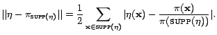
Rather, we measure the bias w.r.t. the distribution
.
Rather, we measure the bias w.r.t. the distribution ![]() conditioned on
selecting a sample in
conditioned on
selecting a sample in
![]() .
Formally, let
.
Formally, let
![]() be the following distribution on
be the following distribution on
![]() :
:
![]() for all
for all
![]() . The sampling
bias of the sampler is defined as the total variation
distance between
. The sampling
bias of the sampler is defined as the total variation
distance between ![]() and
and
![]() :
:
Since the running time of samplers is dominated by the number of search engine queries they make, we define the query cost of a sampler to be the expected number of search engine queries it performs per sample generated.
4 Monte Carlo methods
We briefly review two of the three
Monte Carlo simulation methods we use in this paper: rejection
sampling and the Metropolis-Hastings algorithm. Importance
sampling cannot be used to construct search engine samplers, but
rather only to directly estimate aggregate statistical parameters
of the index. It is described in more detail in the full version
of this paper. For an elaborate treatment of Monte Carlo methods,
refer to the textbook of Liu [19].
The basic question addressed in stochastic simulation is the
following. There is a target distribution ![]() on a space
on a space ![]() , which is hard
to sample from directly. On the other hand, we have an
easy-to-sample trial distribution
, which is hard
to sample from directly. On the other hand, we have an
easy-to-sample trial distribution ![]() available. Simulation
methods enable using samples from
available. Simulation
methods enable using samples from ![]() to simulate sampling from
to simulate sampling from ![]() , or at least to estimate statistical parameters
under the measure
, or at least to estimate statistical parameters
under the measure ![]() .
Simulators need to know the distributions
.
Simulators need to know the distributions ![]() and
and ![]() in
unnormalized form. That is, given any instance
in
unnormalized form. That is, given any instance
![]() ,
they should be able to compute ``weights''
,
they should be able to compute ``weights''
![]() and
and
![]() that
represent the probabilities
that
represent the probabilities
![]() and
and
![]() ,
respectively. By that we mean that there should exist
normalization constants
,
respectively. By that we mean that there should exist
normalization constants
![]() and
and
![]() s.t. for all
s.t. for all
![]() ,
,
![]() and
and
![]() . The
constants
. The
constants
![]() and
and
![]() themselves
need not be known to the simulator. For example, when
themselves
need not be known to the simulator. For example, when ![]() is a uniform
distribution on
is a uniform
distribution on ![]() ,
a possible unnormalized form is
,
a possible unnormalized form is
![]() . In this case the normalization constant is
. In this case the normalization constant is
![]() .
.
Rejection sampling. Rejection sampling [24] assumes
![]() and assumes
knowledge of an envelope constant
and assumes
knowledge of an envelope constant ![]() , which is at least
, which is at least
![]() . The procedure, described in Figure 1, repeatedly calls a sampler
. The procedure, described in Figure 1, repeatedly calls a sampler
![]() that generates samples
that generates samples
![]() from the trial
distribution
from the trial
distribution ![]() , until a sample
is ``accepted''. To decide whether
, until a sample
is ``accepted''. To decide whether
![]() is accepted,
the procedure tosses a coin whose heads probability is
is accepted,
the procedure tosses a coin whose heads probability is
![]() (note that
this expression is always at most 1, due to the property of the
envelope constant).
(note that
this expression is always at most 1, due to the property of the
envelope constant).
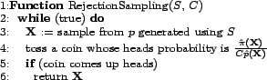
A simple calculation shows that the distribution of the
accepted samples is exactly the target distribution
![]() (hence rejection
sampling yields a perfect sampler). The expected number
of samples from
(hence rejection
sampling yields a perfect sampler). The expected number
of samples from ![]() needed in
order to generate each sample of
needed in
order to generate each sample of ![]() is
is
![]() . Hence, the efficiency of the procedure depends on two factors:
(1) the similarity between the target distribution and the trial
distribution: the more similar they are the smaller is the
maximum
. Hence, the efficiency of the procedure depends on two factors:
(1) the similarity between the target distribution and the trial
distribution: the more similar they are the smaller is the
maximum
![]() ; and (2) the gap between the envelope constant
; and (2) the gap between the envelope constant ![]() and
and
![]() .
.
The Metropolis-Hastings algorithm. The
Metropolis-Hastings (MH) algorithm [21,13] is a Markov Chain Monte Carlo
(MCMC) approach to simulation. Unlike rejection sampling, there
is no single trial distribution, but rather different trial
distributions are used at different steps of the algorithm. The
big advantage over rejection sampling is that no knowledge of an
``envelope constant'' is needed.
The MH algorithm, described in Figure 2,
runs a random walk on ![]() ,
starting from a state
,
starting from a state
![]() . After
. After ![]() steps (called the
``burn-in period''), the reached state is returned as a sample.
The transition probability from state to state is determined by a
``proposal function''
steps (called the
``burn-in period''), the reached state is returned as a sample.
The transition probability from state to state is determined by a
``proposal function'' ![]() , which
is a
, which
is a
![]() stochastic
matrix (i.e., every row of
stochastic
matrix (i.e., every row of ![]() specifies a probability distribution over
specifies a probability distribution over ![]() ). When the random walk reaches a state
). When the random walk reaches a state
![]() , it uses the
distribution specified by the
, it uses the
distribution specified by the
![]() -th row of
-th row of
![]() to choose a ``proposed''
next state
to choose a ``proposed''
next state
![]() . The algorithm
then applies an acceptance-rejection procedure to determine
whether to move to
. The algorithm
then applies an acceptance-rejection procedure to determine
whether to move to
![]() or to stay at
or to stay at
![]() . The
probability of acceptance is:
. The
probability of acceptance is:
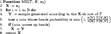
It can be shown that for any proposal function satisfying some
standard restrictions, the resulting random walk converges to
![]() . This means that if
the burn-in period is sufficiently long, the sampling
distribution is guaranteed to be close to
. This means that if
the burn-in period is sufficiently long, the sampling
distribution is guaranteed to be close to ![]() . The convergence rate, i.e., the length of the
burn-in period needed, however, does depend on the proposal
function. There are various algebraic and geometric methods for
figuring out how long should the burn-in period be as a function
of parameters of the proposal function. See a survey by Diaconis
and Saloff-Coste [8] for a
detailed review. If the parameters of the proposal function are
easy to analyze, one can use these methods to set the parameter
. The convergence rate, i.e., the length of the
burn-in period needed, however, does depend on the proposal
function. There are various algebraic and geometric methods for
figuring out how long should the burn-in period be as a function
of parameters of the proposal function. See a survey by Diaconis
and Saloff-Coste [8] for a
detailed review. If the parameters of the proposal function are
easy to analyze, one can use these methods to set the parameter
![]() . Otherwise, empirical
methods are used to set
. Otherwise, empirical
methods are used to set ![]() .
.
Monte Carlo methods with approximate weights. All Monte
Carlo methods assume that the trial distribution ![]() is known, up to
normalization. This assumption turns out to be very problematic
in our setting, since the trial distributions we construct depend
on unknown internal data of the search engine. The best we can do
is come up with an unnormalized weight distribution
is known, up to
normalization. This assumption turns out to be very problematic
in our setting, since the trial distributions we construct depend
on unknown internal data of the search engine. The best we can do
is come up with an unnormalized weight distribution
![]() , whose normalized
form
, whose normalized
form ![]() is statistically close
to
is statistically close
to ![]() . To the best of our
knowledge, no previous study addressed this scenario before.
. To the best of our
knowledge, no previous study addressed this scenario before.
The following theorem proves that as long as ![]() and
and ![]() are close, the sampling
distribution of rejection sampling is close to the target
distribution
are close, the sampling
distribution of rejection sampling is close to the target
distribution ![]() :
:
We believe that similar analysis is possible also for importance sampling and for the Metropolis-Hastings algorithm, but leave it to future work. Nevertheless, our empirical results indicate that these two methods are not significantly affected by the approximate weights.
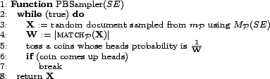
5 Pool-based sampler
In this section we describe our pool-based (PB) sampler. A
query pool is a fragment ![]() of the query space
of the query space ![]() (e.g., all single term queries, all
(e.g., all single term queries, all ![]() -term conjunctions, or
all
-term conjunctions, or
all ![]() -term exact phrases). A
query pool can be constructed by crawling a large corpus of web
documents, such as the ODP directory, and collecting terms or
phrases that occur in its pages. We can run the PB sampler with
any query pool, yet the choice of the pool may affect the
sampling bias, the sampling recall, and the query cost. We
provide quantitative analysis of the impact of various pool
parameters on the PB sampler.
-term exact phrases). A
query pool can be constructed by crawling a large corpus of web
documents, such as the ODP directory, and collecting terms or
phrases that occur in its pages. We can run the PB sampler with
any query pool, yet the choice of the pool may affect the
sampling bias, the sampling recall, and the query cost. We
provide quantitative analysis of the impact of various pool
parameters on the PB sampler.
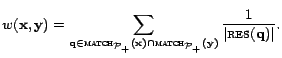
The PB sampler uses as its principal subroutine another
sampler, which generates random documents from ![]() according to the
``match distribution'', which we define below. The match
distribution is non-uniform, yet its unnormalized weights can be
computed efficiently, without submitting queries to the search
engine. Thus, by applying any of the Monte Carlo methods on the
samples from the match distribution, the PB sampler obtains
near-uniform samples. In the analysis below we focus on
application of rejection sampling, due to its simplicity. We note
that the unnormalized weights produced by the PB sampler are only
approximate, hence Theorem 4.1 becomes essential for the
analysis.
according to the
``match distribution'', which we define below. The match
distribution is non-uniform, yet its unnormalized weights can be
computed efficiently, without submitting queries to the search
engine. Thus, by applying any of the Monte Carlo methods on the
samples from the match distribution, the PB sampler obtains
near-uniform samples. In the analysis below we focus on
application of rejection sampling, due to its simplicity. We note
that the unnormalized weights produced by the PB sampler are only
approximate, hence Theorem 4.1 becomes essential for the
analysis.
Preliminaries. ![]() is the
target distribution of the PB sampler. For simplicity of
exposition, we assume
is the
target distribution of the PB sampler. For simplicity of
exposition, we assume ![]() is the
uniform distribution on
is the
uniform distribution on ![]() , although the sampler can be adapted to work for
more general distributions. The unnormalized form of
, although the sampler can be adapted to work for
more general distributions. The unnormalized form of ![]() we use is:
we use is:
![]() , for all
, for all
![]() .
.
![]() is any query
pool. The set of queries
is any query
pool. The set of queries
![]() that overflow (i.e.,
that overflow (i.e.,
![]() ) is denoted
) is denoted
![]() , while the
set of queries
, while the
set of queries
![]() that underflow (i.e.,
that underflow (i.e.,
![]() ) is denoted
) is denoted
![]() . A query that
neither overflows nor underflows is called valid. The
set of valid queries
. A query that
neither overflows nor underflows is called valid. The
set of valid queries
![]() is
denoted
is
denoted
![]() and the set of
invalid queries is denoted
and the set of
invalid queries is denoted
![]() .
.
Let ![]() be any distribution
over
be any distribution
over ![]() . The
overflow probability of
. The
overflow probability of ![]() ,
,
![]() , is
, is
![]() . Similarly, the
underflow probability of
. Similarly, the
underflow probability of ![]() ,
,
![]() , is
, is
![]() .
.
![]() denotes the set of
queries in
denotes the set of
queries in ![]() that a
document
that a
document
![]() matches. That
is,
matches. That
is,
![]() . For example, if
. For example, if ![]() consists of all the 3-term exact phrases, then
consists of all the 3-term exact phrases, then
![]() consists of all the
3-term exact phrases that occur in the document
consists of all the
3-term exact phrases that occur in the document
![]() .
.
We say that ![]() covers a document
covers a document
![]() , if
, if
![]() . Let
. Let
![]() be the
collection of documents covered by
be the
collection of documents covered by ![]() . Note that a sampler that uses only queries
from
. Note that a sampler that uses only queries
from ![]() can never reach
documents outside
can never reach
documents outside
![]() . We thus
define
. We thus
define
![]() to be the
uniform distribution on
to be the
uniform distribution on
![]() . The PB
sampler will generate samples from
. The PB
sampler will generate samples from
![]() and hence
in order to determine its sampling bias, its sampling
distribution will be compared to
and hence
in order to determine its sampling bias, its sampling
distribution will be compared to
![]() .
.
Let ![]() be any distribution
over
be any distribution
over ![]() . The recall of
. The recall of
![]() w.r.t.
w.r.t.
![]() , denoted
, denoted
![]() , is the probability that
a random document selected from
, is the probability that
a random document selected from ![]() is covered by
is covered by ![]() . That is,
. That is,
![]() . The recall of
. The recall of ![]() w.r.t. the uniform distribution is the ratio
w.r.t. the uniform distribution is the ratio
![]() . This recall
will determine the sampling recall of the PB sampler.
. This recall
will determine the sampling recall of the PB sampler.
Match distribution. The match distribution
induced by a query pool ![]() , denoted
, denoted
![]() , is a
distribution over the document collection
, is a
distribution over the document collection ![]() defined as follows:
defined as follows:
![]() . That is, the probability of choosing a document is proportional
to the number of queries from
. That is, the probability of choosing a document is proportional
to the number of queries from ![]() it matches. Note that the support of
it matches. Note that the support of
![]() is exactly
is exactly
![]() .
.
The unnormalized form of
![]() we use is the
following:
we use is the
following:
![]() . We next argue that for ``natural'' query pools,
. We next argue that for ``natural'' query pools,
![]() can be computed
based on the content of
can be computed
based on the content of
![]() alone and
without submitting queries to the search engine. To this
end, we make the following plausible assumption: for any given
document
alone and
without submitting queries to the search engine. To this
end, we make the following plausible assumption: for any given
document
![]() and any
given query
and any
given query
![]() ,
we know, without querying the search engine, whether
,
we know, without querying the search engine, whether
![]() matches
matches
![]() or not. For
example, if
or not. For
example, if ![]() is the set of
single-term queries, then checking whether
is the set of
single-term queries, then checking whether
![]() matches
matches
![]() boils down to
finding the term
boils down to
finding the term
![]() in the text of
in the text of
![]() .
.
Some factors that may impact our ability to determine whether
the search engine matches
![]() with
with
![]() are: (1) How the
search engine pre-processes the document (e.g., whether it
truncates it, if the document is too long). (2) How the search
engine tokenizes the document (e.g., whether it ignores HTML
tags). (3) How the search engine indexes the document (e.g.,
whether it filters out stopwords or whether it indexes also by
anchor text terms). (4) The semantics of the query
are: (1) How the
search engine pre-processes the document (e.g., whether it
truncates it, if the document is too long). (2) How the search
engine tokenizes the document (e.g., whether it ignores HTML
tags). (3) How the search engine indexes the document (e.g.,
whether it filters out stopwords or whether it indexes also by
anchor text terms). (4) The semantics of the query
![]() . Some of the
above are not publicly available. Yet, most search engines follow
standard IR methodologies and reverse engineering work can be
used to learn answers to the above questions.
. Some of the
above are not publicly available. Yet, most search engines follow
standard IR methodologies and reverse engineering work can be
used to learn answers to the above questions.
Since queries typically correspond to the occurrence of terms
or phrases in the document, we can find
![]() , by enumerating the
terms/phrases in
, by enumerating the
terms/phrases in
![]() and deducing the
queries in
and deducing the
queries in ![]() that
that
![]() matches. For
example, if
matches. For
example, if ![]() is the set of
single-term queries, finding all the queries in
is the set of
single-term queries, finding all the queries in ![]() that
that
![]() matches simply
requires finding all the distinct non-stopword terms occurring in
matches simply
requires finding all the distinct non-stopword terms occurring in
![]() .
.
Query volume distribution. A special distribution over a
query pool ![]() is the
query volume distribution, which we denote by
is the
query volume distribution, which we denote by
![]() . The
volume of a query pool
. The
volume of a query pool ![]() , denoted
, denoted
![]() ,
is the sum
,
is the sum
![]() .
.
![]() is defined as:
is defined as:
![]() .
.
The query volume distribution always has an underflow
probability of 0. Yet, the overflow probability may be high,
depending on the pool ![]() .
Typically, there is a tradeoff between this overflow probability
and the the recall of
.
Typically, there is a tradeoff between this overflow probability
and the the recall of ![]() :
the higher the recall, the higher also is the overflow
probability.
:
the higher the recall, the higher also is the overflow
probability.
Note that sampling queries from ![]() according
according
![]() seems hard to
do, since volumes of queries are not known a priori.
seems hard to
do, since volumes of queries are not known a priori.
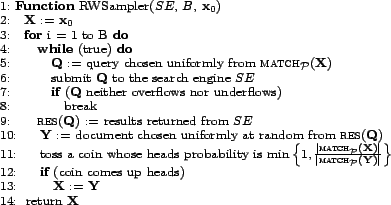
The PB sampler. Assume, for the moment, we have a sampler
![]() that generates
sample documents from the match distribution
that generates
sample documents from the match distribution
![]() . Figure
3 shows our PB sampler, which uses
. Figure
3 shows our PB sampler, which uses
![]() as a
subroutine.
as a
subroutine.
The PB sampler applies rejection sampling with trial
distribution
![]() and target
distribution
and target
distribution
![]() . The
unnormalized weights used for document
. The
unnormalized weights used for document
![]() are
are
![]() and
and
![]() . Since
. Since
![]() is a least
is a least
![]() for any
for any
![]() , then an
envelope constant of
, then an
envelope constant of ![]() is
sufficient. As argued above, we assume the weight
is
sufficient. As argued above, we assume the weight
![]() can be
computed exactly from the content of
can be
computed exactly from the content of
![]() alone. The
following shows that if
alone. The
following shows that if
![]() indeed
generates samples from
indeed
generates samples from
![]() , then the
sampling distribution of the PB sampler is uniform on
, then the
sampling distribution of the PB sampler is uniform on
![]() . The proof
follows directly from the analysis of the rejection sampling
procedure:
. The proof
follows directly from the analysis of the rejection sampling
procedure:
Match distribution sampler. In Figure 4 we describe the match distribution
sampler. For the time being, we make two unrealistic assumptions:
(1) there is a sampler
![]() that samples
queries from the volume distribution
that samples
queries from the volume distribution
![]() ; and (2) the
overflow probability of
; and (2) the
overflow probability of
![]() is 0, although
the pool's recall is high (as argued above, this situation is
unlikely). We later show how to remove these assumptions.
is 0, although
the pool's recall is high (as argued above, this situation is
unlikely). We later show how to remove these assumptions.
The sampler is very similar to the Bharat-Broder sampler,
except that it samples random queries proportionally to their
volume. Since no query overflows, all documents that match a
query are included in its result set. It follows that the
probability of a document to be sampled is proportional to the
number of queries in ![]() that it matches:
that it matches:
We next address the unrealistic assumption that the overflow
probability of
![]() is 0. Rather
than using
is 0. Rather
than using
![]() , which is
likely to have a non-zero overflow probability, we use a
different but related distribution, which is guaranteed to have
an overflow probability of 0. Recall that
, which is
likely to have a non-zero overflow probability, we use a
different but related distribution, which is guaranteed to have
an overflow probability of 0. Recall that
![]() is the set of
valid (i.e., non-overflowing and non-underflowing) queries in
is the set of
valid (i.e., non-overflowing and non-underflowing) queries in
![]() . We can view
. We can view
![]() as a query
pool itself (after all, it is just a set of queries). The volume
distribution
as a query
pool itself (after all, it is just a set of queries). The volume
distribution
![]() of this
pool has, by definition, an overflow probability of 0.
of this
pool has, by definition, an overflow probability of 0.
Suppose we could somehow efficiently sample from
![]() and use
these samples instead of samples from
and use
these samples instead of samples from
![]() . In that
case, by Proposition 5.2, the
sampling distribution
. In that
case, by Proposition 5.2, the
sampling distribution ![]() of the
match distribution sampler equals the match distribution
of the
match distribution sampler equals the match distribution
![]() induced
by the query pool
induced
by the query pool
![]() .
.
Let us return now to the PB sampler. That sampler assumed
![]() generates
samples from
generates
samples from
![]() . What happens
if instead it generates samples from
. What happens
if instead it generates samples from
![]() ? Note
that now there is a mismatch between the trial distribution used
by the PB sampler (i.e.,
? Note
that now there is a mismatch between the trial distribution used
by the PB sampler (i.e.,
![]() ) and the
unnormalized weights it uses (i.e.,
) and the
unnormalized weights it uses (i.e.,
![]() ).
).
One solution could be to try to compute the unnormalized
weights of
![]() , i.e.,
, i.e.,
![]() . However, this seems hard to do efficiently, because
. However, this seems hard to do efficiently, because
![]() is no longer a
``natural'' query pool. In particular, given a document
is no longer a
``natural'' query pool. In particular, given a document
![]() , how do we know
which of the queries that it matches are valid? To this end, we
need to send all the queries in
, how do we know
which of the queries that it matches are valid? To this end, we
need to send all the queries in
![]() to the search engine
and filter out the overflowing queries. This solution incurs a
prohibitively high query cost. Instead, we opt for a different
solution: we leave the PB sampler as is; that is, the trial
distribution will be
to the search engine
and filter out the overflowing queries. This solution incurs a
prohibitively high query cost. Instead, we opt for a different
solution: we leave the PB sampler as is; that is, the trial
distribution will be
![]() but the
unnormalized weights will remain those of
but the
unnormalized weights will remain those of
![]() (i.e.,
(i.e.,
![]() ). This
means that the samples generated by the PB sampler are no longer
truly uniform. The following theorem uses Theorem 4.1 to bound the distance of
these samples from uniformity. It turns out that this distance
depends on two factors: (1) the overflow probability
). This
means that the samples generated by the PB sampler are no longer
truly uniform. The following theorem uses Theorem 4.1 to bound the distance of
these samples from uniformity. It turns out that this distance
depends on two factors: (1) the overflow probability
![]() ; and (2)
; and (2)
![]() , which is the
probability that a random document chosen from
, which is the
probability that a random document chosen from
![]() matches at
least one valid query in
matches at
least one valid query in ![]() .
.
Volume distribution sampler. We are left to show how to
sample queries from the volume distribution
![]() efficiently. Our most crucial observation is the following:
efficiently. Our most crucial observation is the following:
![]() can be
easily computed, up to normalization. Given any query
can be
easily computed, up to normalization. Given any query
![]() , we can submit
, we can submit
![]() to the search
engine and determine whether
to the search
engine and determine whether
![]() or
or
![]() . In the former case we also obtain
. In the former case we also obtain
![]() . This gives the following unnormalized form of
. This gives the following unnormalized form of
![]() :
:
![]() for
for
![]() and
and
![]() for
for
![]() . Since we know
. Since we know
![]() in
unnormalized form, we can apply rejection sampling to queries
sampled from some other, arbitrary, distribution
in
unnormalized form, we can apply rejection sampling to queries
sampled from some other, arbitrary, distribution ![]() on
on ![]() , and obtain
samples from
, and obtain
samples from
![]() .
.
The volume distribution sampler is depicted in Figure 5. The sampler uses another query sampler
![]() that generates samples
from an easy-to-sample-from distribution
that generates samples
from an easy-to-sample-from distribution ![]() on
on ![]() .
.
![]() must satisfy
must satisfy
![]() . (We usually
choose
. (We usually
choose ![]() to be the uniform
distribution on
to be the uniform
distribution on ![]() .)
We assume
.)
We assume ![]() is known in some
unnormalized form
is known in some
unnormalized form
![]() and that a
corresponding envelope constant
and that a
corresponding envelope constant ![]() is given. The target distribution of the rejection
sampling procedure is
is given. The target distribution of the rejection
sampling procedure is
![]() . The
unnormalized form used is the one described above. Figuring out
the unnormalized weight of a query requires only a single query
to the search engine. The following now follows directly from the
correctness of rejection sampling:
. The
unnormalized form used is the one described above. Figuring out
the unnormalized weight of a query requires only a single query
to the search engine. The following now follows directly from the
correctness of rejection sampling:
Analysis. The sampling recall and the sampling bias of
the PB sampler are analyzed in Theorem 5.3.
The query cost is bounded as follows:
Choosing the query pool. We next review the parameters of
the query pool that impact the PB sampler.
(1) Pool's recall. The sampler's recall approximately
equals the pool's recall, so we would like pools with high
recall. In order to guarantee high recall, a pool must consist of
queries that include at least one term/phrase from (almost) every
document in ![]() . Since
overflowing queries are not taken into account, we need these
terms not to be too popular. We can obtain such a collection of
terms/phrases by crawling a large corpus of web documents, such
as the ODP directory.
. Since
overflowing queries are not taken into account, we need these
terms not to be too popular. We can obtain such a collection of
terms/phrases by crawling a large corpus of web documents, such
as the ODP directory.
(2) Overflow probability. The bias of the PB sampler
is approximately proportional to the invalidity probability of
the query volume distribution. We thus need the pool and the
corresponding query volume distribution to have a low overflow
probability. Minimizing this probability usually interferes with
the desire to have high recall, so finding a pool and a
distribution that achieve a good tradeoff between the two is
tricky. ![]() -term conjunctions
or disjunctions are problematic because they suffer from a high
overflow probability. We thus opted for
-term conjunctions
or disjunctions are problematic because they suffer from a high
overflow probability. We thus opted for ![]() -term exact phrases. Our experiments hint that for
-term exact phrases. Our experiments hint that for
![]() , the overflow
probability is tiny. If the phrases are collected from a real
corpus, like ODP, then the underflow probability is also small.
The recall of exact phrases is only a bit lower than that of
conjunctions or disjunctions.
, the overflow
probability is tiny. If the phrases are collected from a real
corpus, like ODP, then the underflow probability is also small.
The recall of exact phrases is only a bit lower than that of
conjunctions or disjunctions.
(3) Average number of matches. The query cost of the
PB sampler is proportional to
![]() . Hence, we would like to find pools for which the number of
matches grows moderately with the document length.
. Hence, we would like to find pools for which the number of
matches grows moderately with the document length. ![]() -term exact phrases are
a good example, because the number of matches w.r.t. them grows
linearly with the document length.
-term exact phrases are
a good example, because the number of matches w.r.t. them grows
linearly with the document length. ![]() -term conjunctions or disjunctions are poor choices,
because there the growth is exponential in
-term conjunctions or disjunctions are poor choices,
because there the growth is exponential in ![]() .
.
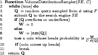
6 Random walk based sampler
The random walk (RW) sampler, described in Figure
6, uses the Metropolis-Hastings algorithm
to perform a random walk on the documents indexed by the search
engine. The graph on these documents is defined by an
implicit query pool ![]() . All we need to know about
. All we need to know about ![]() is how to compute
the match set
is how to compute
the match set
![]() , given a document
, given a document
![]() . We do not need
to know the constituent queries in
. We do not need
to know the constituent queries in ![]() , and thus do not have to crawl a corpus in
order to construct
, and thus do not have to crawl a corpus in
order to construct ![]() .
.
As in the previous section,
![]() denotes the
set of valid queries among the queries in
denotes the
set of valid queries among the queries in ![]() . The graph on
. The graph on ![]() induced by
induced by ![]() ,
which we denote by
,
which we denote by
![]() , is an
undirected weighted graph. The vertex set of
, is an
undirected weighted graph. The vertex set of
![]() is the whole
document collection
is the whole
document collection ![]() . Two
documents
. Two
documents
![]() are
connected by an edge if and only if
are
connected by an edge if and only if
![]() . That is,
. That is,
![]() and
and
![]() are connected
iff there is at least one valid query in
are connected
iff there is at least one valid query in ![]() , which they both match. The weight of the edge
, which they both match. The weight of the edge
![]() is set to be:
is set to be:
Sampling neighbors. We start with the problem of sampling
neighbors according to the proposal function
![]() . To this end, we first come up with following characterization
of vertex degrees:
. To this end, we first come up with following characterization
of vertex degrees:
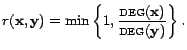
Calculating acceptance probability. Next, we address the
issue of how to calculate the acceptance probability. By
Proposition 6.1, if the current
document is
![]() , and the
proposed neighbor is
, and the
proposed neighbor is
![]() , then the
acceptance probability should be
, then the
acceptance probability should be
![]() . Yet, our sampler cannot know
. Yet, our sampler cannot know
![]() and
and
![]() without submitting queries to the search engine. Instead, it uses
the following perturbed acceptance probability:
without submitting queries to the search engine. Instead, it uses
the following perturbed acceptance probability:
The validity density of a document
![]() is defined
as:
is defined
as:
Why should the variance of the validity density be small? Typically, the validity density of a document is related to the fraction of popular terms occurring in the document. The fraction of popular terms in documents written in the same language (or even in documents written in languages with similar statistical profiles) should be about the same.
Burn-in period. The length of the burn-in period of the
random walk depends on the spectral gap of the Markov
Chain's transition matrix. The difference between the largest and
second largest eigenvalues determines how quickly the random walk
approaches its limit distribution. The bigger the gap, the faster
the convergence. Quantitatively, if we want the distribution of
samples to be at most ![]() away from the limit distribution
away from the limit distribution ![]() , then we need a burn-in period of length
, then we need a burn-in period of length
![]() , where
, where ![]() is the
spectral gap.
is the
spectral gap.
When ![]() is unknown,
one can resort to empirical tests to figure out a sufficient
burn-in period length. One approach is to run the MH algorithm
several times, and empirically find the minimum burn-in period
length
is unknown,
one can resort to empirical tests to figure out a sufficient
burn-in period length. One approach is to run the MH algorithm
several times, and empirically find the minimum burn-in period
length ![]() needed to accurately
estimate statistical parameters of the data whose real value we
somehow know in advance.
needed to accurately
estimate statistical parameters of the data whose real value we
somehow know in advance.
The query cost of the sampler depends on two factors: (1) the
burn-in period ![]() ; and (2) the
validity densities of the documents encountered during the random
walk. When visiting a document
; and (2) the
validity densities of the documents encountered during the random
walk. When visiting a document
![]() , the expected
number of queries selected until hitting a valid query is
, the expected
number of queries selected until hitting a valid query is
![]() , i.e., the inverse validity density of
, i.e., the inverse validity density of
![]() .
.
7 Experimental results
We conducted 3 sets of experiments: (1) pool measurements: estimation of parameters of selected query pools; (2) evaluation experiments: evaluation of the bias of our samplers and the Bharat-Broder (BB) sampler; and (3) exploration experiments: measurements of real search engines.
Experimental setup. For the pool measurements and the
evaluation experiments, we crawled the 3 million pages on the ODP
directory. Of these we kept 2.4 million pages that we could
successfully fetch and parse, that were in text, HTML, or pdf
format, and that were written in English. Each page was given a
serial id, stored locally, and indexed by single terms and
phrases. Only the first 10,000 terms in each page were
considered. Exact phrases were not allowed to cross boundaries,
such as paragraph boundaries.
In our exploration experiments, conducted in January-February 2006, we submitted 220,000 queries to Google, 580,000 queries to MSN Search, and 380,000 queries to Yahoo!. Due to legal limitations on automatic queries, we used the Google, MSN, and Yahoo! web search APIs, which are, reportedly, served from older and smaller indices than the indices used to serve human users.
Our pool measurements and evaluation experiments were performed on a dual Intel Xeon 2.8GHz processor workstation with 2GB RAM and two 160GB disks. Our exploration experiments were conducted on five workstations.
Pool measurements. We selected four candidate query
pools, which we thought could be useful in our samplers: single
terms and exact phrases of lengths 3, 5, and 7. (We measured only
four pools, because each measurement required substantial disk
space and running time.) In order to construct the pools, we
split the ODP data set into two parts: a training set,
consisting of every fifth page (when ordered by id), and a
test set, consisting of the rest of the pages. The pools
were built only from the training data, but the measurements were
done only on the test data. In order to determine whether a query
is overflowing, we set a result limit of ![]() .
.
All our measurements were made w.r.t. the uniform distribution
over the pool (including the overflow probability). Analysis of
the overflow probability of the volume distribution (which is an
important factor in our analysis) will be done in future work.
The results of our measurements are tabulated in Table 1. The normalized deviation of the
validity density is the ratio
![]() , where
, where
![]() is a uniformly
chosen document.
is a uniformly
chosen document.
Table 1: Results of pool parameter measurements
| Parameter | Single terms | Phrases (3) | Phrases (5) | Phrases (7) |
|---|---|---|---|---|
| Size | 2.6M | 97M | 155M | 151M |
| Overflow prob. | 11.4% | 3% | 0.4% | 0.1% |
| Underflow prob. | 40.3% | 56% | 76.2% | 82.1% |
| Recall | 57.6% | 96.5% | 86.7% | 63.9% |
| Avg # of matches | 5.6 | 78.8 | 43.2 | 29 |
| Avg validity density | 2.4% | 29.2% | 55.7% | 67.5% |
| Normalized deviation of validity density | 1.72 | 0.493 | 0.416 | 0.486 |
The measurements show that overflow probability, average number of matches, and average validity density improve as phrase length increases, while recall and underflow probability get worse. The results indicate that a phrase length of 5 achieves the best tradeoff among the parameters. It has a very small overflow probability (less than 0.5%), while maintaining a recall of 86%. The overflow probability of 3-term phrases is a bit too high (3%), while the recall of the 7-term phrases is way too low (about 64%).
Single terms have a relatively low overflow probability, only because we measure the probability w.r.t. the uniform distribution over the terms, and many of the terms are misspellings, technical terms, or digit strings. Note, on the other hand, the minuscule average validity density.
Since the ODP data set is presumably representative of the web, we expect most of these measurements to represent the situation on real search engines. The only exceptions are the overflow and underflow probabilities, which are distorted due to the small size of the ODP data set. We thus measured these parameters on Yahoo!. The results are given in Table 2. It is encouraging to see that for 5-term phrases, the overflow probability remains relatively low, while the underflow probability goes down dramatically. The elevated overflow probability of 3-term phrases is more evident here.
Table 2: Pool parameter measurements on Yahoo!
| Parameter | Single terms | Phrases (3) | Phrases (5) | Phrases (7) |
|---|---|---|---|---|
| Overflow prob. | 40.2% | 15.7% | 2.1% | 0.4% |
| Underflow prob. | 4.5% | 3.4% | 7.2% | 12.9% |
Evaluation experiments. To evaluate our samplers and the BB sampler, we ran them on a home-made search engine built over the ODP data set. In this controlled environment we could compare the sampling results against the real data.
The index of our ODP search engine consisted of the test set
only. It used static ranking by document id to rank query
results. A result limit of ![]() was used in order to have an overflow probability
comparable to the one on Yahoo!.
was used in order to have an overflow probability
comparable to the one on Yahoo!.
We ran four samplers: (1) the PB sampler with rejection sampling; (2) the PB sampler with importance sampling; (3) the RW sampler; and (4) the BB sampler. All the samplers used a query pool of 5-term phrases extracted from the ODP training set. The random walk sampler used a burn-in period of 1,000 steps. Each sampler was allowed to submit exactly 5 million queries to the search engine.
In Figure 7, we show the distribution of samples by document size. We ordered the documents in the index by size, from largest to smallest, and split them into 10 equally sized deciles. Truly uniform samples should distribute evenly among the deciles. The results show the overwhelming difference between our samplers and the BB sampler. The BB sampler generated a huge number of samples at the top decile (more than 50%!). Our samplers had no or little bias.
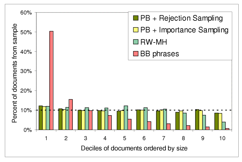
Figure 8 addresses bias towards highly ranked documents. We ordered the documents in the index by their static rank, from highest to lowest, and split into 10 equally sized deciles. The first decile corresponds to the most highly ranked documents. The results indicate that none of our samplers had any significant bias under the ranking criterion. Surprisingly, the BB sampler had bias towards the 4th, 5th, and 6th deciles. When digging into the data, we found that documents whose rank (i.e., id) belonged to these deciles had a higher average size than documents with lower or higher rank. Thus, the bias we see here is in fact an artifact of the bias towards long documents. A good explanation is that our 5-term exact phrases pool had a low overflow probability in the first place, so very few queries overflowed.
We have several conclusions from the above experiments: (1) the 5-term phrases pool, which has small overflow probability, made an across-the-board improvement to all the samplers (including BB). This was evidenced by the lack of bias towards highly ranked documents. (2) The BB sampler suffers from a severe bias towards long documents, regardless of the query pool used. (3) Our pool-based samplers seem to give the best results, showing no bias in any of the experiments. (4) The random walk has a small negative bias towards short documents. Possibly by running the random walk more steps, this negative bias could be alleviated.
Exploration experiments. We used our most successful
sampler, the PB sampler, to generate uniform samples from Google,
MSN Search, and Yahoo!. For complete details of the experimental
setup, see the full version of the paper.
Table 3 tabulates the measured relative sizes of the Google, MSN Search, and Yahoo! indices. Since our query pool consisted mostly of English language phrases, our results refer mainly to the English portion of these indices. We also remind the reader that the indices we experimented with are somewhat outdated. In order to test whether a URL belongs to the index, we used a standard procedure [4,12].
Table 2: Relative sizes of major search engines.
| Pages from
|
MSN | Yahoo! | |
|---|---|---|---|
| 46% | 45% | ||
| MSN | 55% | 51% | |
| Yahoo! | 44% | 22% |
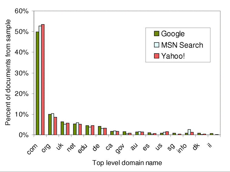
Figure 9 shows the domain name distributions in the three indices. Note that there are some minor differences among the search engines. For example the .info domain is covered much better by MSN Search than by Google and Yahoo!.
8 Conclusions
We presented two novel search engine samplers. The first, the pool-based sampler, provides weights together with the samples, and can thus be used in conjunction with stochastic simulation techniques to produce near-uniform samples. We showed how to apply these simulations even when the weights are approximate. We fully analyzed this sampler and identified the query pool parameters that impact its bias and performance. We then estimated these parameters on real data, consisting of the English pages from the ODP hierarchy, and showed that a pool of 5-term phrases induces nearly unbiased samples. Our second sampler runs a random walk on a graph defined over the index documents. Its primary advantage is that it does not need a query pool. Empirical evidence suggests that the random walk converges quickly to its limit equilibrium distribution. It is left to future work to analyze the spectral gap of this random walk in order to estimate the convergence rate mathematically.
We note that the bias towards English language documents is a limitation of our experimental setup and not of the techniques themselves. The bias could be eliminated by using a more comprehensive dictionary or by starting random walks from pages in different languages.
Finally, we speculate that our methods may be applicable in a more general setting. For example, for sampling from databases, deep web sites, library records, etc.
REFERENCES
[1] A. Anagnostopoulos, A. Broder, and D. Carmel, Sampling search-engine results, In Proc. 14th WWW, pages 245-256, 2005.
[2] Z. Bar-Yossef, A. Berg, S. Chien, J. Fakcharoenphol, and D. Weitz, Approximating aggregate queries about Web pages via random walks, In Proc. 26th VLDB, pages 535-544, 2000.
[3] J. Battelle, John Battelle's searchblog, battellemedia.com/archives/001889.php, 2005.
[4] K. Bharat and A. Broder, A technique for measuring the relative size and overlap of public Web search engines, In Proc. 7th WWW, pages 379-388, 1998.
[5] E. Bradlow and D. Schmittlein, The little engines that could: Modelling the performance of World Wide Web search engines, Marketing Science, 19:43-62, 2000.
[6] F. Can, R. Nuray, and A. B. Sevdik, Automatic performance evaluation of Web search engines, Infor. Processing and Management, 40:495-514, 2004.
[7] M. Cheney and M. Perry, A comparison of the size of the Yahoo! and Google indices, vburton.ncsa.uiuc.edu/indexsize.html, 2005.
[8] P. Diaconis and L. Saloff-Coste, What do we know about the Metropolis algorithm? J. of Computer and System Sciences, 57:20-36, 1998.
[9] dmoz, The open directory project, dmoz.org.
[10] A. Dobra and S. Fienberg, How large is the World Wide Web? Web Dynamics, pages 23-44, 2004.
[11] M. Gordon and P. Pathak, Finding information on the World Wide Web: the retrieval effectiveness of search engines, Information Processing and Management, 35(2):141-180, 1999.
[12] A. Gulli and A. Signorini, The indexable Web is more than 11.5 billion pages, In Proc. 14th WWW (Posters), pages 902-903, 2005.
[13] W. Hastings, Monte Carlo sampling methods using Markov chains and their applications, Biometrika, 57(1):97-109, 1970.
[14] D. Hawking, N. Craswel, P. Bailey, and K. Griffiths, Measuring search engine quality, Information Retrieval, 4(1):33-59, 2001.
[15] M. Henzinger, A. Heydon, M. Mitzenmacher, and M. Najork, Measuring index quality using random walks on the Web, In Proc. 8th WWW, pages 213-225, 1999.
[16] M. Henzinger, A. Heydon, M. Mitzenmacher, and M. Najork, On near-uniform URL sampling, In Proc. 9th WWW, pages 295-308, 2000.
[17] S. Lawrence and C. Giles, Searching the World Wide Web, Science, 5360(280):98, 1998.
[18] S. Lawrence and C. Giles, Accessibility of information on the Web, Nature, 400:107-109, 1999.
[19] J. S. Liu, Monte Carlo Strategies in Scientific Computing, Springer, 2001.
[20] T. Mayer, Our blog is growing up and so has our index, www.ysearchblog.com/archives/000172.html.
[21] N. Metropolis, A. Rosenbluth, M. Rosenbluth, A. Teller, and E. Teller, Equations of state calculations by fast computing machines, J. of Chemical Physics, 21:1087-1091, 1953.
[22] G. Price, More on the total database size battle and Googlewhacking with Yahoo, blog.searchenginewatch.com/blog/050811-231448, 2005.
[23] P. Rusmevichientong, D. Pennock, S. Lawrence, and C. Lee Giles, Methods for sampling pages uniformly from the World Wide Web, In AAAI Fall Symp., 2001.
[24] J. von Neumann, Various techniques used in connection with random digits, In John von Neumann, Collected Works, volume V. Oxford, 1963.