|
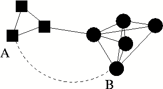
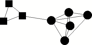
An important characteristic of all SNs is the community graph structure: how social actors gather into groups such that they are intra-group close and inter-group loose [13]. An illustration of a simple two-community SN is sketched in Fig. 1. Here each node represents a social actor in the SN and different node shapes represent different communities. Two nodes share an edge if and only if a relationship exists between them according to social definitions such as their role or participation in the social network. Connections in this case are binary.
Discovering community structures from general networks is of obvious interest. Early methods include graph partitioning [8] and hierarchical clustering [19,25]. Recent algorithms [6,14,2] addressed several problems related to prior knowledge of community size, the precise definition of inter-vertices similarity measure and improved computational efficiency [13]. They have been applied successfully to various areas such as email networks [22] and the Web [5]. Semantic similarity between Web pages can be measured using human-generated topical directories [9]. In general, semantic similarity in SNs is the meaning or reason behind the network connections.
For the extraction of community structures from email corpora [22,3], the social network is usually constructed measuring the intensity of contacts between email users. In this setting, every email user is a social actor, modeled as a node in the SN. An edge between two nodes indicates that the existing email communication between them is higher than certain frequency threshold.
However, discovering a community simply based purely on communication intensity becomes problematic in some scenarios. (1) Consider a spammer in an email system who sends out a large number of messages. There will be edges between every user and the spammer, in theory presenting a problem to all community discovery methods which are topology based. (2) Aside from the possible bias in network topology due to unwanted communication, existing methods also suffer from the lack of semantic interpretation. Given a group of email users discovered as a community, a natural question is why these users form a community? Pure graphical methods based on network topology, without the consideration of semantics, fall short in answering to such questions.
Consider other ways a community can be established, e.g. Fig.
2. From the preset communication
intensity, person ![]() and
person
and
person ![]() belong to two
different communities, denoted by squares and circles, based on a
simple graph partitioning. However, ignoring the document semantics
in their communications, their common interests (denoted by the
dashed line) are not considered in traditional community
discovery.
belong to two
different communities, denoted by squares and circles, based on a
simple graph partitioning. However, ignoring the document semantics
in their communications, their common interests (denoted by the
dashed line) are not considered in traditional community
discovery.
In this paper, we examine the inner community property within SNs by analyzing the semantically rich information, such as emails or documents. We approach the problem of community detection using a generative Bayesian network that models the generation of communication in an SN. As suggested in established social science theory [23], we consider the formation of communities as resulting from the similarity among social actors. The generative models we propose introduce such similarity as a hidden layer in the probabilistic model.
As a parallel study in social network with the sociological approaches, our method advances existing algorithms by not exclusively relying the intensity of contacts. Our approach provides topic tags for every community and corresponding users, giving a semantic description to each community. We test our method on the newly disclosed email corpora benchmark - the Enron email dataset and compare with an existing method.
The outline of this paper is as follows: in Section 2, we introduce the previous work which our models are built on. The community detection problem following the line of probabilistic modeling is explained. Section 3 describes our community-user-topic (CUT) models. In Section 4 we introduce the algorithms of Gibbs sampling and EnF-Gibbs sampling (Gibbs sampling with Entropy Filtering). Experimental results are presented in Section 5. We conclude and discuss future work in Section 6.
|
|
|
| Topic-Word (LDA) | Author-Word | Author-Topic |
Given a set of documents ![]() , each consisting of a sequence of words
, each consisting of a sequence of words ![]() of size
of size
![]() , the generation
of each word
, the generation
of each word
![]() for a specific document
for a specific document ![]() can be
modeled from the perspective of either author or topic, or the
combination of both. Fig. 3 illustrates the
three possibilities using plate notations. Let
can be
modeled from the perspective of either author or topic, or the
combination of both. Fig. 3 illustrates the
three possibilities using plate notations. Let ![]() denote a
specific word observed in document
denote a
specific word observed in document ![]() ;
; ![]() and
and ![]() represent the number
of topics and authors;
represent the number
of topics and authors;
![]() is the
observed set of authors for
is the
observed set of authors for ![]() . Note that the latent variables are light-colored while
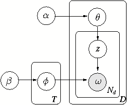
the observed ones are shadowed. Fig. 3(a) models documents as generated by a
mixture of topics [1]. The prior
distributions of topics and words follow Dirichlets parameterized
respectively by
. Note that the latent variables are light-colored while
the observed ones are shadowed. Fig. 3(a) models documents as generated by a
mixture of topics [1]. The prior
distributions of topics and words follow Dirichlets parameterized
respectively by ![]() and
and
![]() . Each topic is a
probabilistic multinomial distribution over words. Let
. Each topic is a
probabilistic multinomial distribution over words. Let ![]() denote the
topic's distributions over words while
denote the
topic's distributions over words while ![]() the document's distribution over topics. 1
the document's distribution over topics. 1
In the Topic-Word model, a document is considered as a mixture
of topics. Each topic corresponds to a multinomial distribution
over the vocabulary. The existence of observed word ![]() in document
in document
![]() is considered to be
drawn from the word distribution
is considered to be
drawn from the word distribution ![]() , which is specific to topic
, which is specific to topic ![]() . Similarly the topic
. Similarly the topic
![]() was drawn from the
document-specific topic distribution
was drawn from the
document-specific topic distribution
![]() , usually a
row in the matrix
, usually a
row in the matrix ![]() .2
.2
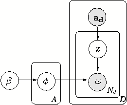
Similar to the Topic-Word model, an Author-Word model
prioritizes the author interest as the origin of a word [11]. In Fig. 3(b),
![]() is the
author set that composes document
is the
author set that composes document ![]() . Each word in this
. Each word in this ![]() is chosen from the author-specific distribution over
words. Note that in this Author-Word model, the author responsible
for a certain word is chosen at random from
is chosen from the author-specific distribution over
words. Note that in this Author-Word model, the author responsible
for a certain word is chosen at random from
![]() .
.
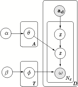
An influential work following this model [21] introduces the Author-Topic model combined with the Topic-Word and Author-Word models and regards the generation of a document as affected by both factors in a hierarchical manner. Fig. 3(c) presents the hierarchical Bayesian structure.
According to the Author-Topic model in Fig. 3(c), for each observed word
![]() in document
in document
![]() , an author
, an author
![]() is drawn uniformly
from the corresponding author group
is drawn uniformly
from the corresponding author group
![]() . Then with
the probability distribution of topics conditioned on
. Then with
the probability distribution of topics conditioned on ![]() ,
,
![]() , a
topic
, a
topic ![]() is generated.
Finally the
is generated.
Finally the ![]() produces
produces
![]() as observed in
document
as observed in
document ![]() .
.
The Author-Topic model has been shown to perform well for document content characterization because it involves two essential factors in producing a general document: the author and the topic. Modeling both factors as variables in the Bayesian network provides the model with capacity to group the words used in a document corpus into semantic topics. Based on the posterior probability obtained after the network is set up, a document can be denoted as a mixture of topic distributions. In addition, each author's preference of using words and involvement in topics can be discovered.
The estimation of the Bayesian network in the aforementioned models typically reply on the observed pairs of author and words in documents. Each word is treated as an instance generated following the probabilistic hierarchy in the models. Some layers in the Bayesian hierarchy are observed, such as authors and words. Other layers are hidden that is to be estimated, such as topics.
Much communication in SNs usually occurs by exchanging documents, such as emails, instant messages or posts on message boards [15]. Such content rich documents naturally serve as an indicator of the innate semantics in the communication among an SN. Consider an information scenario where all communications rely on email. Such email documents usually reflect nearly every aspect of and reasons for this communication. For example, the recipient list records the social actors that are associated with this email and the message body stores the topics they are interested in.
We define such a document carrier of communication as a communication document. Our main contribution is resolving the SN communication modeling problem into the modeling of generation of the communication documents, based on whose features the social actors associate with each other.
Modeling communication based on communication document takes into consideration the semantic information of the document as well as the interactions among social actors. Many features of the SN can be revealed from the parameterized models such as the leader-follower relation [12]. Using such models, we can avoid the effect of meaningless communication documents, such as those generated by a network spammer, in producing communities.
Our models accentuate the impact of community on the SN communications by introducing community as a latent variable in the generative models for communication documents. One direct application of the models is semantic community detection from SNs. Rather than studying network topology, we address the problem of community exploration and generation in SNs following the line of aforementioned research in probabilistic modeling.
We study the community structure of an SN by modeling the communication documents among its social actors and the format of communication documents we model is email because emails embody valuable information regarding shared knowledge and the SN infrastructure [22].
Our Community-User-Topic (CUT) model3 builds on the Author-Topic model. However, the modeling of a communication document includes more factors than the combination of authors and topics.
Serving as an information carrier for communication, a communication document is usually generated to share some information within a group of individuals. But unlike publication documents such as technical reports, journal papers, etc., the communication documents are inaccessible for people who are not in the recipient list. The issue of a communication document indicates the activities of and is also conditioned on the community structure within an SN. Therefore we consider the community as an extra latent variable in the Bayesian network in addition to the author and topic variables. By doing so, we guarantee that the issue of a communication document is purposeful in terms of the existing communities. As a result, the communities in an SN can be revealed and also semantically explanable.
We will use generative Bayesian networks to simulate the generation of emails in SNs. Differing in weighting the impact of a community on users and topics, two versions of CUT are proposed.
We first consider an SN community as no more than a group of
users. This is a notion similar to that assumed in a topology-based
method. For a specific topology-based graph partitioning algorithm
such as
![]() [13], the connection
between two users can be simply weighted by the frequency of their
communications. In our first model CUT
[13], the connection
between two users can be simply weighted by the frequency of their
communications. In our first model CUT![]() , we treat each community as a multinomial distribution
over users. Each user
, we treat each community as a multinomial distribution
over users. Each user ![]() is
associated with a conditional probability
is
associated with a conditional probability ![]() which measures the degree that
which measures the degree that ![]() belongs to community
belongs to community
![]() . The goal is
therefore to find out the conditional probability of a user given
each community. Then users can be tagged with a set of topics, each
of which is a distribution over words. A community discovered by
CUT
. The goal is
therefore to find out the conditional probability of a user given
each community. Then users can be tagged with a set of topics, each
of which is a distribution over words. A community discovered by
CUT![]() is typically in the
structure as shown in Fig. 8.
is typically in the
structure as shown in Fig. 8.
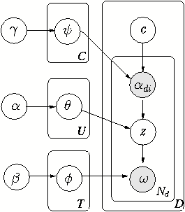
Fig. 4 presents the hierarchy of the
Bayesian network for CUT![]() . Let
us use the same notations in Author-Topic model:
. Let
us use the same notations in Author-Topic model: ![]() and
and ![]() parameterizing
the prior Dirichlets for topics and words. Let
parameterizing
the prior Dirichlets for topics and words. Let ![]() denote the
multinomial distribution over users for each community
denote the
multinomial distribution over users for each community ![]() , each marginal of
which is a Dirichlet parameterized by
, each marginal of
which is a Dirichlet parameterized by ![]() . Let the prior probabilities for
. Let the prior probabilities for ![]() be uniform. Let
be uniform. Let
![]() ,
, ![]() ,
, ![]() denote the number of
community, users and topics.
denote the number of
community, users and topics.
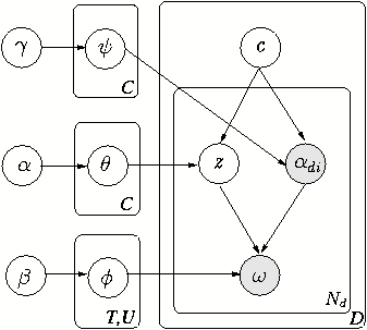
Typically, an email message ![]() is generated by four steps: (1) there is a need for a
community
is generated by four steps: (1) there is a need for a
community ![]() to issue an act
of communication by sending an email
to issue an act
of communication by sending an email ![]() ; (2) a user
; (2) a user ![]() is
chosen from
is
chosen from ![]() as observed in
the recipient list in
as observed in
the recipient list in ![]() ; (3)
; (3)
![]() presents to read
presents to read
![]() since a topic
since a topic
![]() is concerned, which
is drawn from the conditional probability on
is concerned, which
is drawn from the conditional probability on ![]() over topics; (4)
given topic
over topics; (4)
given topic ![]() , a word
, a word
![]() is created in
is created in
![]() . By iterating the
same procedure, an email message
. By iterating the
same procedure, an email message ![]() is composed word by word.
is composed word by word.
Note that the ![]() is not
necessarily the composer of the message in our models. This differs
from existing literatures which assume
is not
necessarily the composer of the message in our models. This differs
from existing literatures which assume ![]() as the author of document. The assumption is that a
user is concerned with any word in a communication document
as long as the user is on the recipient list.
as the author of document. The assumption is that a
user is concerned with any word in a communication document
as long as the user is on the recipient list.
To compute
![]() ,
the posterior probability of assigning each word
,
the posterior probability of assigning each word ![]() to a certain
community
to a certain
community ![]() , user
, user
![]() and topic
and topic
![]() , consider the joint
distribution of all variables in the model:
, consider the joint
distribution of all variables in the model:
Theoretically, the conditional probability
![]() can be computed using the joint distribution
can be computed using the joint distribution
![]() .
.
A possible side-effect of CUT![]() , which considers a community
, which considers a community ![]() solely as a multinomial distribution over users, is
it relaxes the community's impact on the generated topics.
Intrinsically, a community forms because its users communicate
frequently and in addition they share common topics in discussions
as well. In CUT
solely as a multinomial distribution over users, is
it relaxes the community's impact on the generated topics.
Intrinsically, a community forms because its users communicate
frequently and in addition they share common topics in discussions
as well. In CUT![]() where
community only generates users and the topics are generated
conditioned on users, the relaxation is propagated, leading to a
loose connection between community and topic. We will see in the
experiments that the communities discovered by CUT
where
community only generates users and the topics are generated
conditioned on users, the relaxation is propagated, leading to a
loose connection between community and topic. We will see in the
experiments that the communities discovered by CUT![]() is similar to the
topology-based algorithm
is similar to the
topology-based algorithm
![]() proposed in
[13].
proposed in
[13].
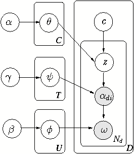
As illustrated in Fig. 5, each word
![]() observed in
email
observed in
email ![]() is finally chosen
from the multinomial distribution of a user
is finally chosen
from the multinomial distribution of a user
![]() , which is
from the recipient list of
, which is
from the recipient list of ![]() . Before that,
. Before that,
![]() is sampled
from another multinomial of topic
is sampled
from another multinomial of topic ![]() and
and ![]() is drawn from
community
is drawn from
community ![]() 's distribution
over topics.
's distribution
over topics.
Analogously, the products of CUT![]() are a set of conditional probability
are a set of conditional probability ![]() that
determines which of the topics are most likely to be discussed in
community
that
determines which of the topics are most likely to be discussed in
community ![]() . Given a topic
group that
. Given a topic
group that ![]() associates for
each topic
associates for
each topic ![]() , the users who
refer to
, the users who
refer to ![]() can be discovered by
measuring
can be discovered by
measuring ![]() .
.
CUT![]() differs from
CUT
differs from
CUT![]() in strengthing the
relation between community and topic. In CUT
in strengthing the
relation between community and topic. In CUT![]() , semantics play a more important role in the
discovery of communities. Similar to CUT
, semantics play a more important role in the
discovery of communities. Similar to CUT![]() , the side-effect of advancing topic
, the side-effect of advancing topic ![]() in the generative
process might lead to loose ties between community and users. An
obvious phenomena of using CUT
in the generative
process might lead to loose ties between community and users. An
obvious phenomena of using CUT![]() is that some users are grouped to the same community
when they share common topics even if they correspond rarely,
leading to the different scenarios for which the CUT models are
most appropriate. For CUT
is that some users are grouped to the same community
when they share common topics even if they correspond rarely,
leading to the different scenarios for which the CUT models are
most appropriate. For CUT![]() ,
users often tend to be grouped to the same communities while
CUT
,
users often tend to be grouped to the same communities while
CUT![]() accentuates the
topic similarities between users even if their communication seem
less frequent.
accentuates the
topic similarities between users even if their communication seem
less frequent.
Derived from Fig. 5, define in
CUT![]() the joint
distribution of community
the joint
distribution of community ![]() , user
, user ![]() , topic
, topic
![]() and word
and word ![]() :
:
Let us see how these models can be used to discover the
communities that consist of users and topics. Consider the
conditional probability
![]() , a
word
, a
word ![]() associates
three variables: community, user and topic. Our interpretation of
the semantic meaning of
associates
three variables: community, user and topic. Our interpretation of
the semantic meaning of
![]() is
the probability that word
is
the probability that word ![]() is generated by user
is generated by user ![]() under topic
under topic ![]() , in
community
, in
community ![]() .
.
Unfortunately, this conditional probability can not be computed
directly. To get
![]() ,we have:
,we have:
Consider the denominator in Eq. 3, summing
over all ![]() ,
, ![]() and
and ![]() makes the
computation impractical in terms of efficiency. In addition, as
shown in [7],
the summing doesn't factorize, which makes the manipulation of
denominator difficult. In the following section, we will show how
an approximate approach of Gibbs sampling will provide solutions to
such problems. A faster algorithm EnF-Gibbs sampling will also be
introduced.
makes the
computation impractical in terms of efficiency. In addition, as
shown in [7],
the summing doesn't factorize, which makes the manipulation of
denominator difficult. In the following section, we will show how
an approximate approach of Gibbs sampling will provide solutions to
such problems. A faster algorithm EnF-Gibbs sampling will also be
introduced.
Gibbs sampling was first introduced to estimate the Topic-Word
model in [7]. In
Gibbs sampling, a Markov chain is formed, the transition between
successive states of which is simulated by repeatedly drawing a
topic for each observed word from its conditional probability on
all other variables. In the Author-Topic model, the algorithm goes
over all documents word by word. For each word
![]() , the topic
, the topic
![]() and the author
and the author
![]() responsible for
this word are assigned based on the posterior probability
conditioned on all other variables:
responsible for
this word are assigned based on the posterior probability
conditioned on all other variables:
![]() .
.
![]() and
and ![]() denote the topic
and author assigned to
denote the topic
and author assigned to
![]() , while
, while
![]() and
and
![]() are all
other assignments of topic and author excluding current instance.
are all
other assignments of topic and author excluding current instance.
![]() represents other observed words in the document set and
represents other observed words in the document set and
![]() is the
observed author set for this document.
is the
observed author set for this document.
A key issue in using Gibbs sampling for distribution
approximation is the evaluation of conditional posterior
probability. In Author-Topic model, given ![]() topics and
topics and ![]() words,
words,
![]() is estimated by:
is estimated by:
The transformation from Eq. 4 to Eq.
5 drops the variables,
![]() ,
,
![]() ,
,
![]() ,
,
![]() , because
each instance of
, because
each instance of ![]() is
assumed independent of the other words in a message.
is
assumed independent of the other words in a message.
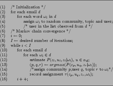
The framework of Gibbs sampling is illustrated in Fig. 6. Given the set of users ![]() , set of email documents
, set of email documents ![]() , the number of desired topic
, the number of desired topic ![]() , number of desired community
, number of desired community ![]() are
input, the algorithm starts with randomly assigning words to a
community, user and topic. A Markov chain is constructed to
converge to the target distribution. In each trial of this Monte
Carlo simulation, a block of
are
input, the algorithm starts with randomly assigning words to a
community, user and topic. A Markov chain is constructed to
converge to the target distribution. In each trial of this Monte
Carlo simulation, a block of
![]() is assigned to the observed word
is assigned to the observed word
![]() . After a
number of states in the chain, the joint distribution
. After a
number of states in the chain, the joint distribution
![]() approximates the targeted distribution.
approximates the targeted distribution.
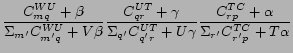
To adapt Gibbs sampling for CUT models, the key step is
estimation of
![]() . For the two CUT models, we
describe the estimation methods respectively.
. For the two CUT models, we
describe the estimation methods respectively.
Let
![]() be the probability that
be the probability that ![]() is generated by community
is generated by community ![]() , user
, user ![]() on
topic
on
topic ![]() , which is
conditioned on all the assignments of words excluding the current
observation of
, which is
conditioned on all the assignments of words excluding the current
observation of ![]() .
.
![]() ,
,
![]() and
and
![]() represent
all the assignments of topic, user and word not including current
assignment of word
represent
all the assignments of topic, user and word not including current
assignment of word ![]() .
.
In CUT![]() , combining Eq.
1 and Eq. 3, assuming
uniform prior probabilities on community
, combining Eq.
1 and Eq. 3, assuming
uniform prior probabilities on community ![]() , we can compute
, we can compute
![]() for CUT
for CUT![]() by:
by:
 |
(7) |
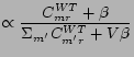
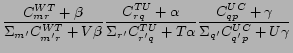
In the equations above,
![]() is the
number of times that word
is the
number of times that word
![]() is assigned
to topic
is assigned
to topic ![]() , not including
the current instance.
, not including
the current instance.
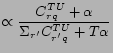
![]() is the
number of times that topic
is the
number of times that topic ![]() is associated with user
is associated with user ![]() and
and
![]() is the
number of times that user
is the
number of times that user ![]() belongs to community
belongs to community ![]() , both not including the current instance.
, both not including the current instance. ![]() is the number of
communities in the social network given as an argument.
is the number of
communities in the social network given as an argument.
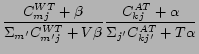
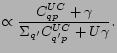
The computation for Eq. 8 requires
keeping a ![]() matrix
matrix
![]() , each entry
, each entry
![]() of which
records the number of times that word
of which
records the number of times that word ![]() is assigned to topic
is assigned to topic ![]() . Similarly, a
. Similarly, a ![]() matrix
matrix ![]() and a
and a ![]() matrix
matrix
![]() are needed for
computation in Eq. 9 and Eq. 10.
are needed for
computation in Eq. 9 and Eq. 10.
Similarly,
![]() is estimated based on the Bayesian structure in CUT
is estimated based on the Bayesian structure in CUT![]() :
:
Hence the computation of CUT![]() demands the storage of three 2-D matrices:
demands the storage of three 2-D matrices: ![]() ,
, ![]() and
and
![]() .
.
With the set of matrices obtained after successive states in the
Markov chain, the semantic communities can be discovered and tagged
with semantic labels. For example, in CUT![]() , the users belonging to each community
, the users belonging to each community ![]() can be discovered by
maximizing
can be discovered by
maximizing ![]() in
in
![]() . Then the
topics that these users concern are similarly obtained from
. Then the
topics that these users concern are similarly obtained from
![]() and
explanation for each topic can be retrieved from
and
explanation for each topic can be retrieved from ![]() .
.
Consider two problems with Gibbs sampling illustrated in Fig.
6: (1) efficiency: Gibbs sampling has been
known to suffer from high computational complexity. Given a textual
corpus with ![]() words. Let
there be
words. Let
there be ![]() users,
users,
![]() communities and
communities and
![]() topics. An
topics. An
![]() iteration
Gibbs sampling has the worst time complexity
iteration
Gibbs sampling has the worst time complexity
![]() , which
in this case is about
, which
in this case is about ![]() computations. (2) performance: unless performed
explicitly before Gibbs sampling, the algorithm may yield poor
performance by including many nondescriptive words. For Gibbs
sampling, some common words like 'the', 'you', 'and' must be
cleaned before Gibbs sampling. However, the EnF-Gibbs sampling
saves such overhead by automatically removing the non-informative
words based on entropy measure.
computations. (2) performance: unless performed
explicitly before Gibbs sampling, the algorithm may yield poor
performance by including many nondescriptive words. For Gibbs
sampling, some common words like 'the', 'you', 'and' must be
cleaned before Gibbs sampling. However, the EnF-Gibbs sampling
saves such overhead by automatically removing the non-informative
words based on entropy measure.
Fig. 7 illustrates the EnF-Gibbs sampling
algorithm we propose. We incorporate the idea of entropy filtering
into Gibbs sampling. During the interactions of EnF-Gibbs sampling,
the algorithm keeps in ![]() an index of words that are not informative. After
an index of words that are not informative. After
![]() times of iterations,
we start to ignore the words that are either already in the
times of iterations,
we start to ignore the words that are either already in the
![]() or are
non-informative. In Step 15 of Fig. 7, we
quantify the informativeness of a word
or are
non-informative. In Step 15 of Fig. 7, we
quantify the informativeness of a word ![]() by the entropy of this word over another variable.
For example, in CUT
by the entropy of this word over another variable.
For example, in CUT![]() where
where
![]() keeps the
numbers of times
keeps the
numbers of times ![]() is
assigned to all topics, we calculate the entropy on the
is
assigned to all topics, we calculate the entropy on the ![]() row of the
matrix.
row of the
matrix.
In this section, we present examples of discovered semantic
communities. Then we compare our communities with those discovered
by the topology-based algorithm
![]() [2] by comparing
groupings of users. Finally we evaluate the computational
complexity of Gibbs sampling and EnF-Gibbs sampling for our
models.
[2] by comparing
groupings of users. Finally we evaluate the computational
complexity of Gibbs sampling and EnF-Gibbs sampling for our
models.
We implemented all algorithms in JAVA and all experiments have been executed on Pentium IV 2.6GHz machines with 1024MB DDR of main memory and Linux as operating system.
In all of our simulations, we fixed the number of communities
![]() at 6 and the number
of topics
at 6 and the number
of topics ![]() at 20. The
smoothing hyper-parameters
at 20. The
smoothing hyper-parameters ![]() ,
, ![]() and
and
![]() were set at
were set at
![]() , 0.01 and 0.1
respectively. We ran 1000 iterations for both our Gibbs sampling
and EnF-Gibbs sampling with the MySQL database support. Because the
quality of results produced by Gibbs sampling and our EnF-Gibbs
sampling are very close, we simply present the results of EnF-Gibbs
sampling hereafter.
, 0.01 and 0.1
respectively. We ran 1000 iterations for both our Gibbs sampling
and EnF-Gibbs sampling with the MySQL database support. Because the
quality of results produced by Gibbs sampling and our EnF-Gibbs
sampling are very close, we simply present the results of EnF-Gibbs
sampling hereafter.
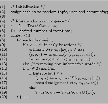
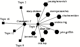
The ontologies for both models are illustrated in Fig. 8 and Fig. 11. In both figures, we
denote user, topic and community by square, hexagon and dot
respectively. In CUT![]() results, a community connects a group of users and each user is
associated with a set of topics. A probability threshold can be set
to tune the number of users and topics desired for description of a
community. In Fig. 8, we present all the users
and two topics of one user for a discovered community. By union all
the topics for the desired users of a community, we can tag a
community with topic labels.
results, a community connects a group of users and each user is
associated with a set of topics. A probability threshold can be set
to tune the number of users and topics desired for description of a
community. In Fig. 8, we present all the users
and two topics of one user for a discovered community. By union all
the topics for the desired users of a community, we can tag a
community with topic labels.
| Topic 3 | Topic 5 | Topic 12 | Topic 14 |
|---|---|---|---|
| rate | dynegy | budget | contract |
| cash | gas | plan | monitor |
| balance | transmission | chart | litigation |
| number | energy | deal | agreement |
| price | transco | project | trade |
| analysis | calpx | report | cpuc |
| database | power | group | pressure |
| deals | california | meeting | utility |
| letter | reliant | draft | materials |
| fax | electric | discussion | citizen |
Fig. 8 shows that user mike.grigsby is one
of the users in community 3. Two of the topics that is mostly
concerned with mike.grigsby are topic 5 and topic 12. Table 1 shows
explanations for some of the topics discovered for this community.
We obtain the word description for a topic by choosing 10 from the
top 20 words that maximize ![]() . We only choose 10 words out of 20 because
there exist some names with large conditional probability on a
topic that for privacy concern we do not want to disclose.
. We only choose 10 words out of 20 because
there exist some names with large conditional probability on a
topic that for privacy concern we do not want to disclose.
| abbreviations | organizations |
|---|---|
| dynegy | An electricity, natural gas provider |
| transco | A gas transportation company |
| calpx | California Power Exchange Corp. |
| cpuc | California Public Utilities Commission |
| ferc | Federal Energy Regulatory Commission |
| epsa | Electric Power Supply Association |
| naruc | National Association of |
| Regulatory Utility Commissioners | |
We can see from Table 1 that words with similar semantics are nicely grouped to the same topics. For better understanding of some abbreviate names popularly used in Enron emails, we list the abbreviations with corresponding complete names in Table 2.
|
[Over communities] 0.35userCom.eps [Over
topics] 0.35harry.arora.eps
|
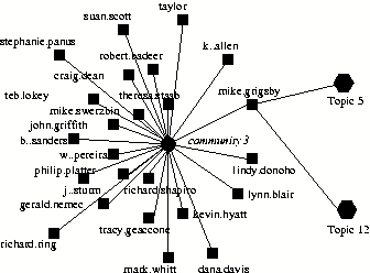
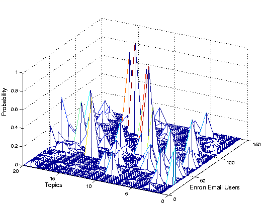
For a single user, Fig. 9 illustrates
its probability distribution over communities and topics as learned
from the CUT![]() model. We can
see the multinomial distribution we assumed was nicely discovered
in both figures. The distribution over topics for all users are
presented in Fig. 10. From Fig. 10, we can see some Enron employees are highly
active to be involved in certain topics while some are relatively
inactive, varying in heights of peaks over users.
model. We can
see the multinomial distribution we assumed was nicely discovered
in both figures. The distribution over topics for all users are
presented in Fig. 10. From Fig. 10, we can see some Enron employees are highly
active to be involved in certain topics while some are relatively
inactive, varying in heights of peaks over users.
Fig. 11 illustrates a community discovered
by CUT![]() . According to the
figure, Topic 8 belongs to the semantic community and this topic
concerns a set of users, which includes rick.buy whose frequently
used words are more or less related to business and risk.
Surprisingly enough, we found the words our CUT
. According to the
figure, Topic 8 belongs to the semantic community and this topic
concerns a set of users, which includes rick.buy whose frequently
used words are more or less related to business and risk.
Surprisingly enough, we found the words our CUT![]() learned to describe
such users were very appropriate after we checked the original
positions of these employees in Enron. For the four users presented
in Table 3, d..steffes was the vice president of Enron in charge of
government affairs; cara.semperger was a senior analyst;
mike.grigsby was a marketing manager and rick.buy was the chief
risk management officer.
learned to describe
such users were very appropriate after we checked the original
positions of these employees in Enron. For the four users presented
in Table 3, d..steffes was the vice president of Enron in charge of
government affairs; cara.semperger was a senior analyst;
mike.grigsby was a marketing manager and rick.buy was the chief
risk management officer.
| d..steffes | cara.s | mike.grigsby | rick.buy |
|---|---|---|---|
| power | number | file | corp |
| transmission | cash | trader | loss |
| epsa | ferc | report | risk |
| ferc | database | price | activity |
| generator | peak | customer | validation |
| government | deal | meeting | off |
| california | bilat | market | business |
| cpuc | caps | sources | possible |
| electric | points | position | increase |
| naruc | analysis | project | natural |
Given ![]() data objects, the
similarity between two clustering results
data objects, the
similarity between two clustering results ![]() is
defined5:
is
defined5:
where ![]() denotes the
count of object pairs that are in different clusters for both
clustering and
denotes the
count of object pairs that are in different clusters for both
clustering and ![]() is the
count of pair that are in the same cluster.
is the
count of pair that are in the same cluster.
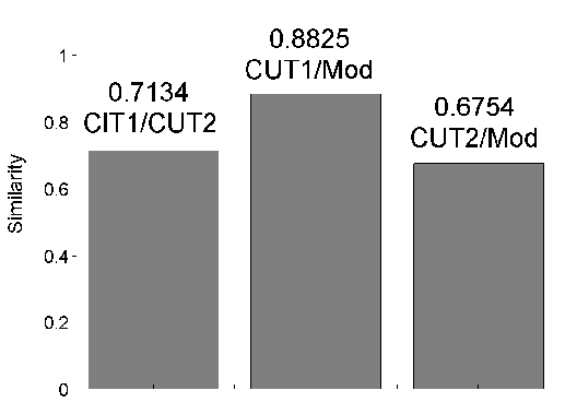
The similarities between three CUT models and
![]() are
illustrated in Fig. 12. We can see that
as we expected the similarity between CUT
are
illustrated in Fig. 12. We can see that
as we expected the similarity between CUT![]() and
and
![]() is large
while that between CUT
is large
while that between CUT![]() and
and
![]() is small.
This is because the CUT
is small.
This is because the CUT![]() is
more similar to
is
more similar to
![]() than
CUT
than
CUT![]() by defining a
community as no more than a group of users.
by defining a
community as no more than a group of users.
We also test the similarity among topics(users) for the
users(topics) which are discovered as a community by CUT![]() (CUT
(CUT![]() ). Typically the
topics(users) associated with the users(topics) in a community
represent high similarities. For example, in Fig. 8, Topic 5 and Topic 12 that concern mike.grigsby are
both contained in the topic set of lindy.donoho, who is the
community companion of mike.grigsby.
). Typically the
topics(users) associated with the users(topics) in a community
represent high similarities. For example, in Fig. 8, Topic 5 and Topic 12 that concern mike.grigsby are
both contained in the topic set of lindy.donoho, who is the
community companion of mike.grigsby.
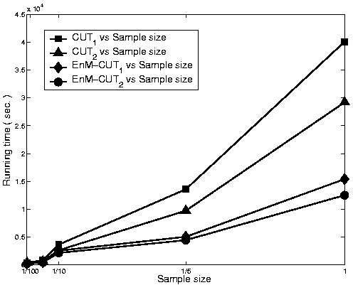
We evaluate the computational complexity of Gibbs sampling and EnF-Gibbs sampling for our models. For the two metrics we measure the computational complexity based on are total running time and iteration-wise running time. For overall running time we sampled different scales of subsets of messages from Enron email corpus. For the iteration-wise evaluation, we ran both Gibbs sampling and EnF-Gibbs sampling on complete dataset.
In Fig. 13(a), the running time of
both sampling algorithms on two models are illustrated. We can see
that generally learning CUT![]() is more efficient than CUT
is more efficient than CUT![]() . It is a reasonable result considering the matrices for
CUT
. It is a reasonable result considering the matrices for
CUT![]() are larger in scales
than CUT
are larger in scales
than CUT![]() . Also entropy
filtering in Gibbs sampling leads to 4 to 5 times speedup
overall.
. Also entropy
filtering in Gibbs sampling leads to 4 to 5 times speedup
overall.
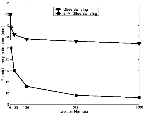
The step-wise running time comparison between Gibbs sampling and EnF-Gibbs sampling is shown in Fig. 13(b). We perform the entropy filtering removal after 8 iterations in the Markov chain. We can see the EnF-Gibbs sampling well outperforms Gibbs sampling in efficiency. Our experimental results also show that the quality of EnF-Gibbs sampling and Gibbs sampling are almost the same.
We present two versions of Community-User-Topic models for semantic community discovery in social networks. Our models combine the generative probabilistic modeling with community detection. To simulate the generative models, we introduce EnF-Gibbs sampling which extends Gibbs sampling based on entropy filtering. Experiments have shown that our method effectively tags communities with topic semantics with better efficiency than Gibbs sampling.
Future work would consider the possible expansion of our CUT models as illustrated in Fig. 14. The two CUT models we proposed either emphasize the relation between community and users or between community and topics. It would be interesting to see how the community structure changes when both factors are simultaneously considered. One would expect new communities to emerge. The model in Fig. 14 constrains the community as a joint distribution over topic and users. However, such nonlinear generative models require larger computational resources, asking for more efficient yet approximate solutions. It would also be interesting to explore the predictive performance of these models on new communications between strange social actors in SNs.