The PageRank algorithm for determining the ``importance'' of Web pages has become a central technique in Web search [18]. The core of the PageRank algorithm involves computing the principal eigenvector of the Markov matrix representing the hyperlink structure of the Web. As the Web graph is very large, containing over a billion nodes, the PageRank vector is generally computed offline, during the preprocessing of the Web crawl, before any queries have been issued.
The development of techniques for computing PageRank efficiently for Web-scale graphs is important for a number of reasons. For Web graphs containing a billion nodes, computing a PageRank vector can take several days. Computing PageRank quickly is necessary to reduce the lag time from when a new crawl is completed to when that crawl can be made available for searching. Furthermore, recent approaches to personalized and topic-sensitive PageRank schemes [11,20,14] require computing many PageRank vectors, each biased towards certain types of pages. These approaches intensify the need for faster methods for computing PageRank.
Eigenvalue computation is a well-studied area of numerical linear algebra for which there exist many fast algorithms. However, many of these algorithms are unsuitable for our problem as they require matrix inversion, a prohibitively costly operation for a Web-scale matrix. Here, we present a series of novel algorithms devised expressly for the purpose of accelerating the convergence of the iterative PageRank computation. We show empirically on an 80 million page Web crawl that these algorithms speed up the computation of PageRank by 25-300%.
In this section we summarize the definition of PageRank [18] and review some of the mathematical tools we will use in analyzing and improving the standard iterative algorithm for computing PageRank.
Underlying the definition of PageRank is the following basic
assumption. A link from a page
![]() to
a page
to
a page
![]() can be viewed as evidence that
can be viewed as evidence that ![]() is an ``important'' page. In particular, the
amount of importance conferred on
is an ``important'' page. In particular, the
amount of importance conferred on ![]() by
by ![]() is proportional to the importance of
is proportional to the importance of ![]() and inversely proportional to
the number of pages
and inversely proportional to
the number of pages ![]() points to. Since the importance of
points to. Since the importance of ![]() is itself not known, determining the
importance for every page
is itself not known, determining the
importance for every page
![]() requires an iterative fixed-point computation.
requires an iterative fixed-point computation.
To allow for a more rigorous analysis of the necessary
computation, we next describe an equivalent formulation in terms of
a random walk on the directed Web graph ![]() . Let
. Let
![]() denote the existence of an edge from
denote the existence of an edge from ![]() to
to ![]() in
in ![]() . Let
. Let
![]() be the
outdegree of page
be the
outdegree of page ![]() in
in
![]() . Consider a random
surfer visiting page
. Consider a random
surfer visiting page ![]() at time
at time ![]() . In the next time step, the surfer chooses a
node
. In the next time step, the surfer chooses a
node ![]() from among
from among ![]() 's out-neighbors
's out-neighbors
![]() uniformly at random.
In other words, at time
uniformly at random.
In other words, at time ![]() , the surfer lands at node
, the surfer lands at node
![]() with
probability
with
probability
![]() .
.
The PageRank of a page ![]() is defined as the probability that at some
particular time step
is defined as the probability that at some
particular time step ![]() , the surfer is at page
, the surfer is at page ![]() . For sufficiently large
. For sufficiently large ![]() , and with minor modifications
to the random walk, this probability is unique, illustrated as
follows. Consider the Markov chain induced by the random walk on
, and with minor modifications
to the random walk, this probability is unique, illustrated as
follows. Consider the Markov chain induced by the random walk on
![]() , where the states
are given by the nodes in
, where the states
are given by the nodes in ![]() , and the stochastic transition matrix
describing the transition from
, and the stochastic transition matrix
describing the transition from ![]() to
to ![]() is given by
is given by ![]() with
with
![]() .
.
For ![]() to
be a valid transition probability matrix, every node must have at
least 1 outgoing transition; i.e.,
to
be a valid transition probability matrix, every node must have at
least 1 outgoing transition; i.e., ![]() should have no rows consisting of all zeros.
This holds if
should have no rows consisting of all zeros.
This holds if ![]() does
not have any pages with outdegree 0,
which does not hold for the Web graph.
does
not have any pages with outdegree 0,
which does not hold for the Web graph. ![]() can be converted into a valid transition
matrix by adding a complete set of outgoing transitions to pages
with outdegree 0. In other words, we can
define the new matrix
can be converted into a valid transition
matrix by adding a complete set of outgoing transitions to pages
with outdegree 0. In other words, we can
define the new matrix ![]() where all states have at least one outgoing
transition in the following way. Let
where all states have at least one outgoing
transition in the following way. Let ![]() be the number of nodes (pages) in the Web
graph. Let
be the number of nodes (pages) in the Web
graph. Let ![]() be the
be the ![]() -dimensional column vector representing a
uniform probability distribution over all nodes:
-dimensional column vector representing a
uniform probability distribution over all nodes:
Let ![]() be the
be the ![]() -dimensional column vector identifying the
nodes with outdegree 0:
-dimensional column vector identifying the
nodes with outdegree 0:
|
Then we construct ![]() as
follows:
as
follows:
In terms of the random walk, the effect of ![]() is to modify the transition
probabilities so that a surfer visiting a dangling page (i.e., a
page with no outlinks) randomly jumps to another page in the next
time step, using the distribution given by
is to modify the transition
probabilities so that a surfer visiting a dangling page (i.e., a
page with no outlinks) randomly jumps to another page in the next
time step, using the distribution given by ![]() .
.
By the Ergodic Theorem for Markov chains [9], the Markov chain defined by
![]() has a unique
stationary probability distribution if
has a unique
stationary probability distribution if ![]() is aperiodic and irreducible; the former
holds for the Markov chain induced by the Web graph. The latter
holds iff
is aperiodic and irreducible; the former
holds for the Markov chain induced by the Web graph. The latter
holds iff ![]() is
strongly connected, which is generally not the case for
the Web graph. In the context of computing PageRank, the standard
way of ensuring this property is to add a new set of complete
outgoing transitions, with small transition probabilities, to
all nodes, creating a complete (and thus strongly
connected) transition graph. In matrix notation, we construct the
irreducible Markov matrix
is
strongly connected, which is generally not the case for
the Web graph. In the context of computing PageRank, the standard
way of ensuring this property is to add a new set of complete
outgoing transitions, with small transition probabilities, to
all nodes, creating a complete (and thus strongly
connected) transition graph. In matrix notation, we construct the
irreducible Markov matrix ![]() as follows:
as follows:
In terms of the random walk, the effect of ![]() is as follows. At each time
step, with probability
is as follows. At each time
step, with probability ![]() , a surfer visiting any node will jump to a
random Web page (rather than following an outlink). The destination
of the random jump is chosen according to the probability
distribution given in
, a surfer visiting any node will jump to a
random Web page (rather than following an outlink). The destination
of the random jump is chosen according to the probability
distribution given in ![]() . Artificial jumps taken because of
. Artificial jumps taken because of ![]() are referred to as
teleportation.
are referred to as
teleportation.
By redefining the vector ![]() given in Equation 1 to be nonuniform, so that
given in Equation 1 to be nonuniform, so that ![]() and
and ![]() add artificial transitions with nonuniform
probabilities, the resultant PageRank vector can be biased to
prefer certain kinds of pages. For this reason, we refer to
add artificial transitions with nonuniform
probabilities, the resultant PageRank vector can be biased to
prefer certain kinds of pages. For this reason, we refer to ![]() as the
personalization vector.
as the
personalization vector.
For simplicity and consistency with prior work, the remainder of
the discussion will be in terms of the transpose matrix,
![]() ; i.e.,
the transition probability distribution for a surfer at node
; i.e.,
the transition probability distribution for a surfer at node ![]() is given by row
is given by row ![]() of
of ![]() , and column
, and column ![]() of
of ![]() .
.
Note that the edges artificially introduced by ![]() and
and ![]() never need to be explicitly materialized, so
this construction has no impact on efficiency or the sparsity of
the matrices used in the computations. In particular, the
matrix-vector multiplication
never need to be explicitly materialized, so
this construction has no impact on efficiency or the sparsity of
the matrices used in the computations. In particular, the
matrix-vector multiplication
![]() can be implemented efficiently using Algorithm 1.
can be implemented efficiently using Algorithm 1.
Assuming that the probability distribution over the surfer's
location at time 0 is given by
![]() , the
probability distribution for the surfer's location at time
, the
probability distribution for the surfer's location at time ![]() is given by
is given by
![]() . The unique
stationary distribution of the Markov chain is defined as
. The unique
stationary distribution of the Markov chain is defined as
![]() , which is equivalent
to
, which is equivalent
to
![]() , and is
independent of the initial distribution
, and is
independent of the initial distribution
![]() . This
is simply the principal eigenvector of the matrix
. This
is simply the principal eigenvector of the matrix ![]() , which is exactly the
PageRank vector we would like to compute.
, which is exactly the
PageRank vector we would like to compute.
The standard PageRank algorithm computes the principal
eigenvector by starting with
![]() and computing successive
iterates
and computing successive
iterates
![]() until
convergence. This is known as the Power Method, and is discussed in
further detail in Section 3.
until
convergence. This is known as the Power Method, and is discussed in
further detail in Section 3.
While many algorithms have been developed for fast eigenvector computations, many of them are unsuitable for this problem because of the size and sparsity of the Web matrix (see Section 7.1 for a discussion of this).
In this paper, we develop a fast eigensolver, based on the Power
Method, that is specifically tailored to the PageRank problem and
Web-scale matrices. This algorithm, called Quadratic Extrapolation,
accelerates the convergence of the Power Method by periodically
subtracting off estimates of the nonprincipal eigenvectors from the
current iterate
![]() . In
Quadratic Extrapolation, we take advantage of the fact that the
first eigenvalue of a Markov matrix is known to be 1 to compute
estimates of the nonprincipal eigenvectors using successive
iterates of the Power Method. This allows seamless integration into
the standard PageRank algorithm. Intuitively, one may think of
Quadratic Extrapolation as using successive iterates generated by
the Power Method to extrapolate the value of the principal
eigenvector.
. In
Quadratic Extrapolation, we take advantage of the fact that the
first eigenvalue of a Markov matrix is known to be 1 to compute
estimates of the nonprincipal eigenvectors using successive
iterates of the Power Method. This allows seamless integration into
the standard PageRank algorithm. Intuitively, one may think of
Quadratic Extrapolation as using successive iterates generated by
the Power Method to extrapolate the value of the principal
eigenvector.
In the following sections, we will be introducing a series of algorithms for computing PageRank, and discussing the rate of convergence achieved on realistic datasets. Our experimental setup was as follows. We used two datasets of different sizes for our experiments. The STANFORD.EDU link graph was generated from a crawl of the stanford.edu domain created in September 2002 by the Stanford WebBase project. This link graph contains roughly 280,000 nodes, with 3 million links, and requires 12MB of storage. We used STANFORD.EDU while developing the algorithms, to get a sense for their performance. For real-world, Web-scale performance measurements, we used the LARGEWEB link graph, generated from a large crawl of the Web that had been created by the Stanford WebBase project in January 2001 [13]. LARGEWEB contains roughly 80M nodes, with close to a billion links, and requires 3.6GB of storage. Both link graphs had dangling nodes removed as described in [18]. The graphs are stored using an adjacency list representation, with pages represented by 4-byte integer identifiers. On an AMD Athlon 1533MHz machine with a 6-way RAID-5 disk volume and 2GB of main memory, each application of Algorithm 1 on the 80M page LARGEWEB dataset takes roughly 10 minutes. Given that computing PageRank generally requires up to 100 applications of Algorithm 1, the need for fast methods is clear.
We measured the relative rates of convergence of the algorithms
that follow using the L![]() norm of the residual vector; i.e.,
norm of the residual vector; i.e.,
We describe why the L![]() residual is an appropriate measure in Section 6.
residual is an appropriate measure in Section 6.
One way to compute the stationary distribution of a Markov chain
is by explicitly computing the distribution at successive time
steps, using
![]() , until the
distribution converges.
, until the
distribution converges.
This leads us to Algorithm 2, the
Power Method for computing the principal eigenvector of ![]() . The Power Method is the
oldest method for computing the principal eigenvector of a matrix,
and is at the heart of both the motivation and implementation of
the original PageRank algorithm (in conjunction with
Algorithm 1).
. The Power Method is the
oldest method for computing the principal eigenvector of a matrix,
and is at the heart of both the motivation and implementation of
the original PageRank algorithm (in conjunction with
Algorithm 1).
The intuition behind the convergence of the power method is as
follows. For simplicity, assume that the start vector
![]() lies
in the subspace spanned by the eigenvectors of
lies
in the subspace spanned by the eigenvectors of ![]() .
.![[*]](footnote.png) Then
Then
![]() can be
written as a linear combination of the eigenvectors of
can be
written as a linear combination of the eigenvectors of ![]() :
:
| (2) |
Since we know that the first eigenvalue of a Markov matrix is
![]() ,
,
| (3) |
and
| (4) |
Since
![]() ,
,
![]() approaches
approaches ![]() as
as ![]() grows large. Therefore, the Power Method
converges to the principal eigenvector of the Markov matrix
grows large. Therefore, the Power Method
converges to the principal eigenvector of the Markov matrix ![]() .
.
A single iteration of the Power Method consists of the single
matrix-vector multiply
![]() .
Generally, this is an
.
Generally, this is an ![]() operation. However, if the matrix-vector
multiply is performed as in Algorithm 1, the matrix
operation. However, if the matrix-vector
multiply is performed as in Algorithm 1, the matrix ![]() is so sparse that the
matrix-vector multiply is essentially
is so sparse that the
matrix-vector multiply is essentially ![]() . In particular, the average outdegree of
pages on the Web has been found to be around 7 [16]. On our datasets, we
observed an average of around 8 outlinks per page.
. In particular, the average outdegree of
pages on the Web has been found to be around 7 [16]. On our datasets, we
observed an average of around 8 outlinks per page.
It should be noted that if ![]() is close to 1, then the power method
is slow to converge, because
is close to 1, then the power method
is slow to converge, because ![]() must be large before
must be large before
![]() is close
to 0, and vice versa.
is close
to 0, and vice versa.
As we show in [12], the eigengap
![]() for the Web Markov
matrix
for the Web Markov
matrix ![]() is
given exactly by the teleport probability
is
given exactly by the teleport probability ![]() . Thus, when the teleport probability is
large, and the personalization vector
. Thus, when the teleport probability is
large, and the personalization vector ![]() is uniform over all pages, the Power
Method works reasonably well. However, for a large teleport
probability (and with a uniform personalization vector
is uniform over all pages, the Power
Method works reasonably well. However, for a large teleport
probability (and with a uniform personalization vector ![]() ), the effect of link
spam is increased, and pages can achieve unfairly high rankings.
In the extreme case, for a teleport probability of
), the effect of link
spam is increased, and pages can achieve unfairly high rankings.
In the extreme case, for a teleport probability of ![]() , the assignment of rank
to pages becomes uniform. Chakrabarti et al. [5] suggest that
, the assignment of rank
to pages becomes uniform. Chakrabarti et al. [5] suggest that ![]() should be tuned based on the
connectivity of topics on the Web. Such tuning has generally not
been possible, as the convergence of PageRank slows down
dramatically for small values of
should be tuned based on the
connectivity of topics on the Web. Such tuning has generally not
been possible, as the convergence of PageRank slows down
dramatically for small values of ![]() (i.e., values of
(i.e., values of ![]() close to 1).
close to 1).
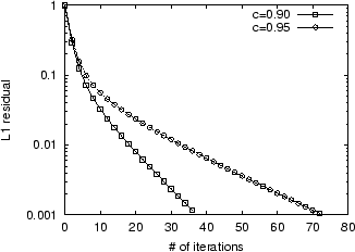
In Figure 1, we show the
convergence on the LARGEWEB dataset
of the Power Method for
![]() using a uniform
using a uniform ![]() . Note that increasing
. Note that increasing ![]() slows down convergence. Since
each iteration of the Power Method takes 10 minutes, computing 100
iterations requires over 16 hours. As the full Web is estimated to
contain over two billion static pages, using the Power Method on
Web graphs close to the size of the Web would require several days
of computation.
slows down convergence. Since
each iteration of the Power Method takes 10 minutes, computing 100
iterations requires over 16 hours. As the full Web is estimated to
contain over two billion static pages, using the Power Method on
Web graphs close to the size of the Web would require several days
of computation.
In the next sections, we describe how to remove the error
components of ![]() along the direction of
along the direction of ![]() and
and ![]() , thus increasing the
effectiveness of Power Method iterations.
, thus increasing the
effectiveness of Power Method iterations.
 |
We begin by introducing an algorithm which we shall call Aitken
Extrapolation. We develop Aitken Extrapolation as follows. We
assume that the iterate
![]() can
be expressed as a linear combination of the first two eigenvectors.
This assumption allows us to solve for the principal eigenvector
can
be expressed as a linear combination of the first two eigenvectors.
This assumption allows us to solve for the principal eigenvector
![]() in closed
form using the successive iterates
in closed
form using the successive iterates
![]() .
.
Of course,
![]() can
only be approximated as a linear combination of the first two
eigenvectors, so the
can
only be approximated as a linear combination of the first two
eigenvectors, so the ![]() that we compute is only an estimate of
the true
that we compute is only an estimate of
the true ![]() . However, it can be seen from
section 3.1 that this
approximation becomes increasingly accurate as
. However, it can be seen from
section 3.1 that this
approximation becomes increasingly accurate as ![]() becomes larger.
becomes larger.
We begin our formulation of Aitken Extrapolation by assuming
that
![]() can
be expressed as a linear combination of the first two
eigenvectors.
can
be expressed as a linear combination of the first two
eigenvectors.
Since the first eigenvalue ![]() of a Markov matrix is
of a Markov matrix is ![]() , we can write the next two
iterates as:
, we can write the next two
iterates as:
Now, let us define
where ![]() represents the
represents the ![]() th
component of the vector
th
component of the vector ![]() . Doing simple algebra using
equations 6 and 7 gives:
. Doing simple algebra using
equations 6 and 7 gives:
| (10) | |||
| (11) |
Now, let us define ![]() as the quotient
as the quotient ![]() :
:
|
(12) | ||
| (13) |
Therefore,
| (14) |
Hence, from equation 5, we have a
closed-form solution for ![]() :
:
However, since this solution is based on the assumption that
![]() can
be written as a linear combination of
can
be written as a linear combination of ![]() and
and ![]() , equation 15 gives only an approximation to
, equation 15 gives only an approximation to
![]() .
Algorithm 3 and Algorithm 4 show how to use Aitken Extrapolation
in conjunction with the Power Method to get consistently better
estimates of
.
Algorithm 3 and Algorithm 4 show how to use Aitken Extrapolation
in conjunction with the Power Method to get consistently better
estimates of ![]() .
.
Aitken Extrapolation is equivalent to applying the well-known
Aitken ![]() method for accelerating linearly
convergent sequences [1] to each component of the
iterate
method for accelerating linearly
convergent sequences [1] to each component of the
iterate
![]() .
What is novel here is this derivation of Aitken acceleration, and
the proof that Aitken acceleration computes the principal
eigenvector of a Markov matrix in one step under the assumption
that the power-iteration estimate
.
What is novel here is this derivation of Aitken acceleration, and
the proof that Aitken acceleration computes the principal
eigenvector of a Markov matrix in one step under the assumption
that the power-iteration estimate
![]() can
be expressed as a linear combination of the first two
eigenvectors.
can
be expressed as a linear combination of the first two
eigenvectors.
As a sidenote, let us briefly develop a related method. Rather
than using equation 8, let us define
![]() alternatively
as:
alternatively
as:
We define ![]() as
in equation 9, and
as
in equation 9, and ![]() now becomes
now becomes
|
|||
By equation 6,
Again, this is an approximation to ![]() , since it's based on the assumption
that
, since it's based on the assumption
that
![]() can
be expressed as a linear combination of
can
be expressed as a linear combination of ![]() and
and ![]() . What is interesting here is that this
is equivalent to performing a second-order epsilon acceleration
algorithm [22] on
each component of the iterate
. What is interesting here is that this
is equivalent to performing a second-order epsilon acceleration
algorithm [22] on
each component of the iterate
![]() . For
this reason, we call this algorithm Epsilon Extrapolation.
. For
this reason, we call this algorithm Epsilon Extrapolation.
In order for an extrapolation method such as Aitken
Extrapolation or Epsilon Extrapolation to be useful, the overhead
should be minimal. By overhead, we mean any costs in addition to
the cost of applying Algorithm 1
to generate iterates. It is clear from inspection that the
operation count of the loop in Algorithm 3 is ![]() , where
, where ![]() is the number of pages on the Web. The
operation count of one extrapolation step is less than the
operation count of a single iteration of the Power Method, and
since Aitken Extrapolation may be applied only periodically, we say
that Aitken Extrapolation has minimal overhead. In our
implementation, the additional cost of each application of Aitken
Extrapolation was negligible - about 1% of the cost of a single
iteration of the Power Method (i.e., 1% of the cost of
Algorithm 1).
is the number of pages on the Web. The
operation count of one extrapolation step is less than the
operation count of a single iteration of the Power Method, and
since Aitken Extrapolation may be applied only periodically, we say
that Aitken Extrapolation has minimal overhead. In our
implementation, the additional cost of each application of Aitken
Extrapolation was negligible - about 1% of the cost of a single
iteration of the Power Method (i.e., 1% of the cost of
Algorithm 1).
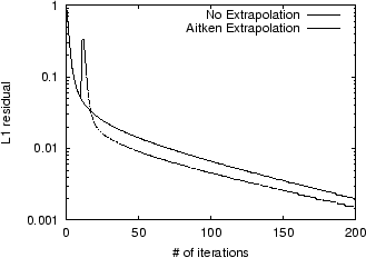
In Figure 2, we show the
convergence of the Power Method with Aitken Extrapolation applied
once at the 10th iteration, compared to the convergence of the
unaccelerated Power Method for the STANFORD.EDU
dataset. The ![]() -axis denotes the number of times a
multiplication
-axis denotes the number of times a
multiplication ![]() occurred; i.e., the number of times
Algorithm 1 was needed. Note that
there is a spike at the acceleration step, but speedup occurs
nevertheless. This spike is caused by the poor approximation for
occurred; i.e., the number of times
Algorithm 1 was needed. Note that
there is a spike at the acceleration step, but speedup occurs
nevertheless. This spike is caused by the poor approximation for
![]() .
.
 |
For ![]() , Aitken Extrapolation takes 38% less time
to reach an iterate with a residual of
, Aitken Extrapolation takes 38% less time
to reach an iterate with a residual of ![]() . However, after this initial speedup, the
convergence rate for Aitken slows down, so that to reach an iterate
with a residual of
. However, after this initial speedup, the
convergence rate for Aitken slows down, so that to reach an iterate
with a residual of ![]() , the time savings drops to 13%. For lower
values of
, the time savings drops to 13%. For lower
values of ![]() ,
Aitken provided much less benefit. Since there is a spike in the
residual graph, if Aitken Extrapolation is applied too often, the
power iterations will not converge. In experiments, Epsilon
Extrapolation performed similarly to Aitken Extrapolation.
,
Aitken provided much less benefit. Since there is a spike in the
residual graph, if Aitken Extrapolation is applied too often, the
power iterations will not converge. In experiments, Epsilon
Extrapolation performed similarly to Aitken Extrapolation.
In this section, we presented Aitken Extrapolation, and a
closely related method called Epsilon Extrapolation. Aitken
Extrapolation is equivalent to applying the well-known Aitken ![]() method [1] to each component of the
iterate
method [1] to each component of the
iterate
![]() , and
Epsilon Extrapolation is equivalent to applying a second-order
epsilon acceleration method to each component of the iterate
, and
Epsilon Extrapolation is equivalent to applying a second-order
epsilon acceleration method to each component of the iterate
![]() [22]. What is novel here is
this derivation of these methods, and the proof that these methods
compute the principal eigenvector of a Markov matrix in one step
under the assumption that the power-iteration estimate
[22]. What is novel here is
this derivation of these methods, and the proof that these methods
compute the principal eigenvector of a Markov matrix in one step
under the assumption that the power-iteration estimate
![]() can
be expressed as a linear combination of the first two eigenvectors.
Furthermore, these methods have not been used thus far to
accelerate eigenvector computations.
can
be expressed as a linear combination of the first two eigenvectors.
Furthermore, these methods have not been used thus far to
accelerate eigenvector computations.
These methods are very different from standard fast eigensolvers, which generally rely strongly on matrix factorizations or matrix inversions. Standard fast eigensolvers do not work well for the PageRank problem, since the web hyperlink matrix is so large and sparse. For problems where the matrix is small enough for an efficient inversion, standard eigensolvers such as inverse iteration are likely to be faster than these methods. The Aitken and Epsilon Extrapolation methods take advantage of the fact that the first eigenvalue of the Markov hyperlink matrix is 1 to find an approximation to the principal eigenvector.
In the next section, we present Quadratic Extrapolation, which
assumes the iterate can be expressed as a linear combination of the
first three eigenvectors, and solves for ![]() in closed form under
this assumption. As we shall soon discuss, the Quadratic
Extrapolation step is simply a linear combination of successive
iterates, and thus does not produce spikes in the residual.
in closed form under
this assumption. As we shall soon discuss, the Quadratic
Extrapolation step is simply a linear combination of successive
iterates, and thus does not produce spikes in the residual.
We develop the Quadratic Extrapolation algorithm as follows. We
assume that the Markov matrix ![]() has only 3 eigenvectors, and that the iterate
has only 3 eigenvectors, and that the iterate
![]() can
be expressed as a linear combination of these 3 eigenvectors. These
assumptions allow us to solve for the principal
eigenvector
can
be expressed as a linear combination of these 3 eigenvectors. These
assumptions allow us to solve for the principal
eigenvector ![]() in closed form using the successive
iterates
in closed form using the successive
iterates
![]() .
.
Of course, ![]() has
more than 3 eigenvectors, and
has
more than 3 eigenvectors, and
![]() can
only be approximated as a linear combination of the first three
eigenvectors. Therefore, the
can
only be approximated as a linear combination of the first three
eigenvectors. Therefore, the ![]() that we compute in this algorithm is
only an estimate for the true
that we compute in this algorithm is
only an estimate for the true ![]() . We show empirically that this
estimate is a better estimate to
. We show empirically that this
estimate is a better estimate to ![]() than the iterate
than the iterate
![]() , and
that our estimate becomes closer to the true value of
, and
that our estimate becomes closer to the true value of ![]() as
as ![]() becomes larger. In
Section 5.3 we show that by
periodically applying Quadratic Extrapolation to the successive
iterates computed in PageRank, for values of
becomes larger. In
Section 5.3 we show that by
periodically applying Quadratic Extrapolation to the successive
iterates computed in PageRank, for values of ![]() close to 1, we can speed up
the convergence of PageRank by a factor of over 3.
close to 1, we can speed up
the convergence of PageRank by a factor of over 3.
We begin our formulation of Quadratic Extrapolation by assuming
that ![]() has only three
eigenvectors
has only three
eigenvectors
![]() and approximating
and approximating
![]() as a
linear combination of these three eigenvectors.
as a
linear combination of these three eigenvectors.
| (16) |
We then define the successive iterates
Since we assume ![]() has
3 eigenvectors, the characteristic polynomial
has
3 eigenvectors, the characteristic polynomial
![]() is
given by:
is
given by:
![]() is a Markov
matrix, so we know that the first eigenvalue
is a Markov
matrix, so we know that the first eigenvalue
![]() . The
eigenvalues of
. The
eigenvalues of ![]() are
also the zeros of the characteristic polynomial
are
also the zeros of the characteristic polynomial
![]() .
Therefore,
.
Therefore,
The Cayley-Hamilton Theorem states that any matrix ![]() satisfies it's own
characteristic polynomial
satisfies it's own
characteristic polynomial ![]() [8]. Therefore, by the
Cayley-Hamilton Theorem, for any vector
[8]. Therefore, by the
Cayley-Hamilton Theorem, for any vector ![]() in
in
![]() ,
,
| (22) |
Letting
![]() ,
,
| (23) |
| (24) |
From equation 21,
We may rewrite this as,
Let us make the following definitions:
| (25) | |||
| (26) | |||
| (27) |
We can now write equation 26 in matrix notation:
We now wish to solve for
![]() . Since
we're not interested in the trivial solution
. Since
we're not interested in the trivial solution
![]() , we
constrain the leading term of the characteristic polynomial
, we
constrain the leading term of the characteristic polynomial ![]() :
:
We may do this because constraining a single coefficient of the
polynomial does not affect the zeros.
Equation 30 is therefore
written:
| (30) |
This is an overdetermined system, so we solve the corresponding least-squares problem.
where ![]() is the
pseudoinverse of the matrix
is the
pseudoinverse of the matrix
![]() . Now, equations 31, 33, and 21
completely determine the coefficients of the characteristic
polynomial
. Now, equations 31, 33, and 21
completely determine the coefficients of the characteristic
polynomial
![]() (equation 20).
(equation 20).
We may now divide
![]() by
by
![]() to get the
polynomial
to get the
polynomial
![]() , whose
roots are
, whose
roots are ![]() and
and ![]() , the second two eigenvalues of
, the second two eigenvalues of ![]() .
.
|
(32) |
Simple polynomial division gives the following values for
![]() and
and ![]() :
:
| (33) | |||
| (34) | |||
| (35) |
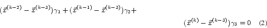
Again, by the Cayley-Hamilton Theorem, if ![]() is any vector in
is any vector in
![]() ,
,
| (36) |
where ![]() is the
eigenvector of
is the
eigenvector of ![]() corresponding to eigenvalue 1 (the principal eigenvector). Letting
corresponding to eigenvalue 1 (the principal eigenvector). Letting
![]() ,
,
| (37) |
From equations 17-19, we get a closed form solution for
![]() :
:
However, since this solution is based on the assumption that ![]() has only 3 eigenvectors,
equation 40 gives only an
approximation to
has only 3 eigenvectors,
equation 40 gives only an
approximation to ![]() .
.
Algorithms 5
and 6 show how to use Quadratic
Extrapolation in conjunction with the Power Method to get
consistently better estimates of ![]() .
.
The overhead in performing the extrapolation shown in
Algorithm 5 comes
primarily from the least-squares computation of ![]() and
and ![]() :
:
It is clear that the other steps in this algorithm are either ![]() or
or ![]() operations.
operations.
Since ![]() is
an
is
an
![]() matrix,
we can do the least-squares solution cheaply in just 2 iterations
of the Gram-Schmidt algorithm [21]. Therefore,
matrix,
we can do the least-squares solution cheaply in just 2 iterations
of the Gram-Schmidt algorithm [21]. Therefore, ![]() and
and ![]() can be computed in
can be computed in
![]() operations.
While a presentation of Gram-Schmidt is outside of the scope of
this paper, we show in Algorithm 7 how to apply Gram-Schmidt to
solve for
operations.
While a presentation of Gram-Schmidt is outside of the scope of
this paper, we show in Algorithm 7 how to apply Gram-Schmidt to
solve for
![]() in
in ![]() operations. Since the extrapolation step is
on the order of a single iteration of the Power Method, and since
Quadratic Extrapolation is applied only periodically during the
Power Method, we say that Quadratic Extrapolation has minimal
overhead. In our experimental setup, the overhead of a single
application of Quadratic Extrapolation is half the cost of a
standard power iteration (i.e., half the cost of Algorithm 1). This number includes the cost of
storing on disk the intermediate data required by Quadratic
Extrapolation (such as the previous iterates), since they may not
fit in main memory.
operations. Since the extrapolation step is
on the order of a single iteration of the Power Method, and since
Quadratic Extrapolation is applied only periodically during the
Power Method, we say that Quadratic Extrapolation has minimal
overhead. In our experimental setup, the overhead of a single
application of Quadratic Extrapolation is half the cost of a
standard power iteration (i.e., half the cost of Algorithm 1). This number includes the cost of
storing on disk the intermediate data required by Quadratic
Extrapolation (such as the previous iterates), since they may not
fit in main memory.
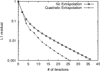
Of the algorithms we have discussed for accelerating the
convergence of PageRank, Quadratic Extrapolation performs the best
empirically. In particular, Quadratic Extrapolation considerably
improves convergence relative to the Power Method when the damping
factor ![]() is
close to 1. We measured the performance of Quadratic Extrapolation
under various scenarios on the
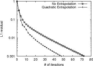
LARGEWEB dataset. Figure 3 shows the rates of convergence
when
is
close to 1. We measured the performance of Quadratic Extrapolation
under various scenarios on the
LARGEWEB dataset. Figure 3 shows the rates of convergence
when ![]() ; after
factoring in overhead, Quadratic Extrapolation reduces the time
needed to reach a residual of
; after
factoring in overhead, Quadratic Extrapolation reduces the time
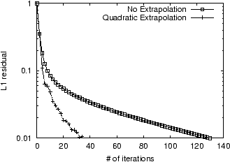
needed to reach a residual of ![]() by 23%.Figure 4 shows the rates of convergence
when
by 23%.Figure 4 shows the rates of convergence
when ![]() ; in this
case, Quadratic Extrapolation speeds up convergence more
significantly, saving 31% in the time needed to reach a residual of
; in this
case, Quadratic Extrapolation speeds up convergence more
significantly, saving 31% in the time needed to reach a residual of
![]() . Finally, in
the case where
. Finally, in
the case where ![]() , the speedup is more dramatic.
Figure 5 shows the rates
of convergence of the Power Method and Quadratic Extrapolation for
, the speedup is more dramatic.
Figure 5 shows the rates
of convergence of the Power Method and Quadratic Extrapolation for
![]() . Because the
Power Method is so slow to converge in this case, we plot the
curves until a residual of
. Because the
Power Method is so slow to converge in this case, we plot the
curves until a residual of ![]() is reached. The use of extrapolation saves
69% in time needed to reach a residual of
is reached. The use of extrapolation saves
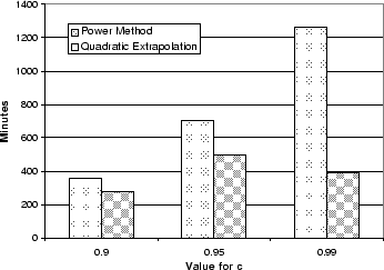
69% in time needed to reach a residual of ![]() ; i.e., the unaccelerated Power Method took
over 3 times as long as the Quadratic Extrapolation method to reach
the desired residual. The wallclock times for each of these
scenarios are summarized in Figure 6.
; i.e., the unaccelerated Power Method took
over 3 times as long as the Quadratic Extrapolation method to reach
the desired residual. The wallclock times for each of these
scenarios are summarized in Figure 6.
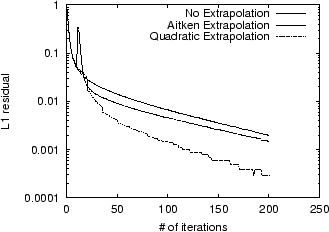
Figure 7 shows the
convergence for the Power Method, Aitken Extrapolation, and
Quadratic Extrapolation on the STANFORD.EDU dataset;
each method was carried out to 200 iterations. To reach a residual
of ![]() , Quadratic
Extrapolation saved 59% in time over the Power Method, as opposed
to a 38% savings for Aitken Extrapolation.
, Quadratic
Extrapolation saved 59% in time over the Power Method, as opposed
to a 38% savings for Aitken Extrapolation.
 |
 |
 |
 |
 |
An important observation about Quadratic Extrapolation is that it does not necessarily need to be applied too often to achieve maximum benefit. By contracting the error in the current iterate along the direction of the second and third eigenvectors, Quadratic Extrapolation actually enhances the convergence of future applications of the standard Power Method. The Power Method, as discussed previously, is very effective in annihilating error components of the iterate in directions along eigenvectors with small eigenvalues. By subtracting off approximations to the second and third eigenvectors, Quadratic Extrapolation leaves error components primarily along the smaller eigenvectors, which the Power Method is better equipped to eliminate.
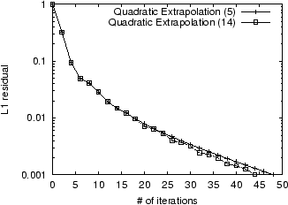
For instance, in Figure 8,
we plot the convergence when Quadratic Extrapolation is applied 5
times compared with when it is applied as often as possible (in
this case, 14 times), to achieve a residual of ![]() . Note that the additional
applications of Quadratic Extrapolation do not lead to much further
improvement. In fact, once we factor in the 0.5 iteration-cost of
each application of Quadratic Extrapolation, the case where it was
applied 5 times ends up being faster.
. Note that the additional
applications of Quadratic Extrapolation do not lead to much further
improvement. In fact, once we factor in the 0.5 iteration-cost of
each application of Quadratic Extrapolation, the case where it was
applied 5 times ends up being faster.
Like Aitken and Epsilon Extrapolation, Quadratic Extrapolation
makes the assumption that an iterate can be expressed as a linear
combination of a subset of the eigenvectors of ![]() in order to find an
approximation to the principal eigenvector of
in order to find an
approximation to the principal eigenvector of ![]() . In Aitken and Epsilon
Extrapolation, we assume that
. In Aitken and Epsilon
Extrapolation, we assume that
![]() can
be written as a linear combination of the first two eigenvectors,
and in Quadratic Extrapolation, we assume that
can
be written as a linear combination of the first two eigenvectors,
and in Quadratic Extrapolation, we assume that
![]() can
be written as a linear combination of the first three eigenvectors.
Since the assumption made in Quadratic Extrapolation is closer to
reality, the resulting approximations are closer to the true value
of the principal eigenvector of
can
be written as a linear combination of the first three eigenvectors.
Since the assumption made in Quadratic Extrapolation is closer to
reality, the resulting approximations are closer to the true value
of the principal eigenvector of ![]() .
.
While Aitken and Epsilon Extrapolation are logical extensions of existing acceleration algorithms, Quadratic Extrapolation is completely novel. Furthermore, all of these algorithms are general purpose. That is, they can be used to compute the principal eigenvector of any large, sparse Markov matrix, not just the web graph. They should be useful in any situation where the size and sparsity of the matrix is such that a QR factorization is prohibitively expensive.
One thing that is interesting to note is that since acceleration
may be applied periodically during any iterative process that
generates iterates
![]() that
converge to the principal eigenvector
that
converge to the principal eigenvector ![]() , it is straightforward to use
Quadratic Extrapolation in conjunction with other methods for
accelerating PageRank, such as Gauss-Seidel [8,2].
, it is straightforward to use
Quadratic Extrapolation in conjunction with other methods for
accelerating PageRank, such as Gauss-Seidel [8,2].
 |
In this section, we present empirical results demonstrating the
suitability of the L![]() residual, even in the context of measuring convergence of
induced document rankings. In measuring the convergence of
the PageRank vector, prior work has usually relied on
residual, even in the context of measuring convergence of
induced document rankings. In measuring the convergence of
the PageRank vector, prior work has usually relied on
![]() ,
the L
,
the L![]() norm of the
residual vector, for
norm of the
residual vector, for ![]() or
or ![]() , as an indicator
of convergence. Given the intended application, we might expect
that a better measure of convergence is the distance, using an
appropriate measure of distance, between the rank orders for query
results induced by
, as an indicator
of convergence. Given the intended application, we might expect
that a better measure of convergence is the distance, using an
appropriate measure of distance, between the rank orders for query
results induced by ![]() and
and ![]() . We use two measures of distance for
rank orders, both based on the the Kendall's-
. We use two measures of distance for
rank orders, both based on the the Kendall's-![]() rank correlation measure:
the
rank correlation measure:
the ![]() measure,
defined below, and the
measure,
defined below, and the ![]() measure, introduced by Fagin et al.
in [7]. To see if the
residual is a ``good'' measure of convergence, we compared it to
the
measure, introduced by Fagin et al.
in [7]. To see if the
residual is a ``good'' measure of convergence, we compared it to
the ![]() and
and ![]() of rankings generated by
of rankings generated by
![]() and
and ![]() .
.
We show empirically that in the case of PageRank computations,
the L![]() residual
residual ![]() is closely correlated
with the
is closely correlated
with the ![]() and
and ![]() distances between query results generated
using the values in
distances between query results generated
using the values in ![]() and
and ![]() .
.
We define the distance measure, ![]() as follows. Consider two partially
ordered lists of URLs,
as follows. Consider two partially
ordered lists of URLs, ![]() and
and ![]() , each of length
, each of length ![]() . Let
. Let ![]() be the union of the URLs in
be the union of the URLs in ![]() and
and ![]() . If
. If ![]() is
is
![]() , then let
, then let
![]() be the
extension of
be the
extension of ![]() , where
, where ![]() contains
contains ![]() appearing after all the URLs in
appearing after all the URLs in ![]() .
We extend
.
We extend ![]() analogously to yield
analogously to yield ![]() .
. ![]() is then defined as:
is then defined as:
| (39) |
In other words,
![]() is the probability that
is the probability that
![]() and
and ![]() disagree
on the relative ordering of a randomly selected pair of distinct
nodes
disagree
on the relative ordering of a randomly selected pair of distinct
nodes
![]() .
.
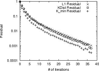
To measure the convergence of PageRank iterations in terms of
induced rank orders, we measured the ![]() distance between the induced rankings
for the top 100 results, averaged across 27 test queries, using
successive power iterates for the
LARGEWEB dataset, with the damping
factor
distance between the induced rankings
for the top 100 results, averaged across 27 test queries, using
successive power iterates for the
LARGEWEB dataset, with the damping
factor ![]() set
to 0.9.The
average residuals using the
set
to 0.9.The
average residuals using the ![]() ,
, ![]() , and L
, and L![]() measures are plotted in Figure 9.
Surprisingly, the L
measures are plotted in Figure 9.
Surprisingly, the L![]() residual is almost perfectly correlated with
residual is almost perfectly correlated with ![]() , and is closely
correlated with
, and is closely
correlated with ![]() .
A rigorous explanation for the close match between the L
.
A rigorous explanation for the close match between the L![]() residual and the Kendall's
residual and the Kendall's
![]() based residuals
is an interesting avenue of future investigation.
based residuals
is an interesting avenue of future investigation.
 |
The field of numerical linear algebra is a mature field, and
many algorithms have been developed for fast eigenvector
computations. However, many of these algorithms are unsuitable for
this problem, because they require matrix inversions or matrix
decompositions that are prohibitively expensive (both in terms of
size and space) for a matrix of the size and sparsity of the
Web-link matrix. For example, inverse iteration will find
the principal eigenvector of ![]() in one iteration, since we know the first
eigenvalue. However, inverse iteration requires the inversion of
in one iteration, since we know the first
eigenvalue. However, inverse iteration requires the inversion of
![]() , which is an
, which is an ![]() operation. The QR
Algorithm with shifts is also a standard fast method for
solving nonsymmetric eigenvalue problems. However, the QR Algorithm
requires a QR factorization of
operation. The QR
Algorithm with shifts is also a standard fast method for
solving nonsymmetric eigenvalue problems. However, the QR Algorithm
requires a QR factorization of ![]() at each iteration, which is also an
at each iteration, which is also an ![]() operation. The
Arnoldi algorithm is also often used for nonsymmetric
eigenvalue problems. However, the strength of Arnoldi is that it
quickly computes estimates to the first few eigenvalues. Once it
has a good estimate of the eigenvalues, it uses inverse iteration
to find the corresponding eigenvectors. In the PageRank problem, we
know that the first eigenvalue of
operation. The
Arnoldi algorithm is also often used for nonsymmetric
eigenvalue problems. However, the strength of Arnoldi is that it
quickly computes estimates to the first few eigenvalues. Once it
has a good estimate of the eigenvalues, it uses inverse iteration
to find the corresponding eigenvectors. In the PageRank problem, we
know that the first eigenvalue of ![]() is 1, since
is 1, since ![]() is a Markov matrix, so we don't need Arnoldi
to give us an estimate of
is a Markov matrix, so we don't need Arnoldi
to give us an estimate of ![]() . For a comprehensive review of these
methods, see [8].
. For a comprehensive review of these
methods, see [8].
However, there is a class of methods from numerical linear
algebra that are useful for this problem. We may rewrite the
eigenproblem
![]() as
the linear system of equations:
as
the linear system of equations:
![]() , and
use the classical iterative methods for linear systems: Jacobi,
Gauss-Seidel, and Successive Overrelaxation (SOR). For the matrix
, and
use the classical iterative methods for linear systems: Jacobi,
Gauss-Seidel, and Successive Overrelaxation (SOR). For the matrix
![]() in the PageRank
problem, the Jacobi method is equivalent to the Power method, but
Gauss-Seidel is guaranteed to be faster. This has been shown
empirically for the PageRank problem [2]. Note, however, that to use
Gauss-Seidel, we would have to sort the adjacency-list
representation of the Web graph, so that back-links for pages,
rather than forward-links, are stored consecutively. The myriad of
multigrid methods are also applicable to this problem. For a review
of multigrid methods, see [17].
in the PageRank
problem, the Jacobi method is equivalent to the Power method, but
Gauss-Seidel is guaranteed to be faster. This has been shown
empirically for the PageRank problem [2]. Note, however, that to use
Gauss-Seidel, we would have to sort the adjacency-list
representation of the Web graph, so that back-links for pages,
rather than forward-links, are stored consecutively. The myriad of
multigrid methods are also applicable to this problem. For a review
of multigrid methods, see [17].
Seminal algorithms for graph analysis for Web-search were introduced by Page et al. [18] (PageRank) and Kleinberg [15] (HITS). Much additional work has been done on improving these algorithms and extending them to new search and text mining tasks [4,6,19,3,20,11]. More applicable to our work are several papers which discuss the computation of PageRank itself [10,2,14]. Haveliwala [10] explores memory-efficient computation, and suggests using induced orderings, rather than residuals, to measure convergence. Arasu et al. [2] uses the Gauss-Seidel method to speed up convergence, and looks at possible speed-ups by exploiting structural properties of the Web graph. Jeh and Widom [14] explore the use of dynamic programming to compute a large number of personalized PageRank vectors simultaneously. Our work is the first to exploit extrapolation techniques specifically designed to speed up the convergence of PageRank, with very little overhead.
Web search has become an integral part of modern information access, posing many interesting challenges in developing effective and efficient strategies for ranking search results. One of the most well-known Web-specific ranking algorithms is PageRank - a technique for computing the authoritativeness of pages using the hyperlink graph of the Web. Although PageRank is largely an offline computation, performed while preprocessing and indexing a Web crawl before any queries have been issued, it has become increasingly desirable to speed up this computation. Rapidly growing crawl repositories, increasing crawl frequencies, and the desire to generate multiple topic-based PageRank vectors for each crawl are all motivating factors for our work in speeding up PageRank computation.
Quadratic Extrapolation is an implementationally simple technique that requires little additional infrastructure to integrate into the standard Power Method. No sorting or modifications of the massive Web graph are required. Additionally, the extrapolation step need only be applied periodically to enhance the convergence of PageRank. In particular, Quadratic Extrapolation works by eliminating the bottleneck for the Power Method, namely the second and third eigenvector components in the current iterate, thus boosting the effectiveness of the simple Power Method itself.
We would like to acknowledge Ronald Fagin for useful discussions
regarding the ![]() measure.
measure.
This paper is based on work supported in part by the National Science Foundation under Grant No. IIS-0085896 and Grant No. CCR-9971010, and in part by the Research Collaboration between NTT Communication Science Laboratories, Nippon Telegraph and Telephone Corporation and CSLI, Stanford University (research project on Concept Bases for Lexical Acquisition and Intelligently Reasoning with Meaning).
![\begin{algorithm} % latex2html id marker 186 [t] $\vec{y} = cP^T\vec{x}$\; $w = ... ... \vec{y} + w \vec{v}$\; \caption{Computing $\vec{y} = A\vec{x}$} \end{algorithm}](img100.png)
![\begin{algorithm} % latex2html id marker 516 [t] function $\vec{x}^{(n)} = \mbox... ...{(k-1)}\vert\vert _1$\; $k = k+1$\; } \} \caption{Power Method} \end{algorithm}](img136.png)
![\begin{algorithm} % latex2html id marker 805 [t] function $\vec{x}^* = \mbox{\te... ... $x_i^*=x_i^{(k)}-g_i/h_i$\; } \} \caption{Aitken Extrapolation} \end{algorithm}](img222.png)
![\begin{algorithm} % latex2html id marker 824 [t] function $\vec{x}^{(n)} = \mbox... ...k = k+1$\; } \} \caption{Power Method with Aitken Extrapolation} \end{algorithm}](img223.png)
![\begin{algorithm} % latex2html id marker 1266 [t] function $\vec{x}^* = \mbox{\t... ...} + \beta_2\vec{x}^{(k)}$\; \} \caption{Quadratic Extrapolation} \end{algorithm}](img335.png)
![\begin{algorithm} % latex2html id marker 1302 [t] function $\vec{x}^{(n)} = \mbo... ... k+1$\; } \} \caption{Power Method with Quadratic Extrapolation} \end{algorithm}](img336.png)
![\begin{algorithm} % latex2html id marker 1335 [t] 1. Compute the reduced $QR$\ f... ...ion{Using Gram-Schmidt to solve for $\gamma_1$\ and $\gamma_2$.} \end{algorithm}](img349.png)