1. Introduction and Motivation
General web search is performed predominantly through text queries to search
engines. Because of the enormous size of the web, text alone is usually not
selective enough to limit the number of query results to a manageable size.
The PageRank algorithm [11], among others
[9], has been proposed (and implemented in
Google [1]) to exploit the linkage structure of the web to
compute global ``importance'' scores that can be used to influence the
ranking of search results. To encompass different notions of importance for
different users and queries, the basic PageRank algorithm can be modified to
create ``personalized views'' of the web, redefining importance according to
user preference. For example, a user may wish to specify his bookmarks as a
set of preferred pages, so that any query results that are important with
respect to his bookmarked pages would be ranked higher. While
experimentation with the use of personalized PageRank has shown its utility
and promise [5,11], the size of the web makes its practical
realization extremely difficult. To see why, let us review the intuition
behind the PageRank algorithm and its extension for personalization.
The fundamental motivation underlying PageRank is the recursive notion that
important pages are those linked-to by many important pages. A page with
only two in-links, for example, may seem unlikely to be an important page,
but it may be important if the two referencing pages are Yahoo! and
Netscape, which themselves are important pages because they have
numerous in-links. One way to formalize this recursive notion is to use the
``random surfer'' model introduced in [11]. Imagine that trillions
of random surfers are browsing the web: if at a certain time step a
surfer is looking at page  , at the next time step he looks at a random
out-neighbor of . As time goes on, the expected percentage of surfers at
each page converges (under certain conditions) to a limit
, at the next time step he looks at a random
out-neighbor of . As time goes on, the expected percentage of surfers at
each page converges (under certain conditions) to a limit  that is
independent of the distribution of starting points. Intuitively, this limit
is the PageRank of , and is taken to be an importance score for ,
since it reflects the number of people expected to be looking at at any
one time.
that is
independent of the distribution of starting points. Intuitively, this limit
is the PageRank of , and is taken to be an importance score for ,
since it reflects the number of people expected to be looking at at any
one time.
The PageRank score reflects a ``democratic'' importance that has no
preference for any particular pages. In reality, a user may have a set  of preferred pages (such as his bookmarks) which he considers more
interesting. We can account for preferred pages in the random surfer model
by introducing a ``teleportation'' probability
of preferred pages (such as his bookmarks) which he considers more
interesting. We can account for preferred pages in the random surfer model
by introducing a ``teleportation'' probability  : at each step, a surfer
jumps back to a random page in with probability , and with
probability
: at each step, a surfer
jumps back to a random page in with probability , and with
probability  continues forth along a hyperlink. The limit distribution
of surfers in this model would favor pages in , pages linked-to by ,
pages linked-to in turn, etc. We represent this distribution as a
personalized PageRank vector (PPV) personalized on the set
. Informally, a PPV is a personalized view of the importance of pages on
the web. Rankings of a user's text-based query results can be biased
according to a PPV instead of the global importance distribution.
continues forth along a hyperlink. The limit distribution
of surfers in this model would favor pages in , pages linked-to by ,
pages linked-to in turn, etc. We represent this distribution as a
personalized PageRank vector (PPV) personalized on the set
. Informally, a PPV is a personalized view of the importance of pages on
the web. Rankings of a user's text-based query results can be biased
according to a PPV instead of the global importance distribution.
Each PPV is of length  , where is the number of pages on
the web. Computing a PPV naively using a fixed-point iteration requires
multiple scans of the web graph [11], which makes it impossible to
carry out online in response to a user query. On the other hand, PPV's for
all preference sets, of which there are
, where is the number of pages on
the web. Computing a PPV naively using a fixed-point iteration requires
multiple scans of the web graph [11], which makes it impossible to
carry out online in response to a user query. On the other hand, PPV's for
all preference sets, of which there are  , is far too large to compute
and store offline. We present a method for encoding PPV's as
partially-computed, shared vectors that are practical to compute and store
offline, and from which PPV's can be computed quickly at query time.
, is far too large to compute
and store offline. We present a method for encoding PPV's as
partially-computed, shared vectors that are practical to compute and store
offline, and from which PPV's can be computed quickly at query time.
In our approach we restrict preference sets to subsets of a set of
hub pages  , selected as those of greater interest for personalization. In
practice, we expect to be a set of pages with high PageRank (``important
pages''), pages in a human-constructed directory such as Yahoo! or
Open Directory [2], or pages important to a
particular enterprise or application. The size of can be thought of as
the available degree of personalization. We present algorithms that, unlike
previous work [5,11], scale well with the size of .
Moreover, the same techniques we introduce can yield approximations on the
much broader set of all PPV's, allowing at least some level of
personalization on arbitrary preference sets.
, selected as those of greater interest for personalization. In
practice, we expect to be a set of pages with high PageRank (``important
pages''), pages in a human-constructed directory such as Yahoo! or
Open Directory [2], or pages important to a
particular enterprise or application. The size of can be thought of as
the available degree of personalization. We present algorithms that, unlike
previous work [5,11], scale well with the size of .
Moreover, the same techniques we introduce can yield approximations on the
much broader set of all PPV's, allowing at least some level of
personalization on arbitrary preference sets.
The main contributions of this paper are as follows.
- A method, based on new graph-theoretical results (listed next), of
encoding PPV's as partial quantities, enabling an efficient,
scalable computation that can be divided between precomputation time and
query time, in a customized fashion according to available resources and
application requirements.
- Three main theorems: The Linearity Theorem allows every PPV to
be represented as a linear combination of basis vectors, yielding a
natural way to construct PPV's from shared components. The Hubs
Theorem allows basis vectors to be encoded as partial vectors
and a hubs skeleton, enabling basis vectors themselves to be
constructed from common components. The Decomposition Theorem
establishes a linear relationship among basis vectors, which is exploited to
minimize redundant computation.
- Several algorithms for computing basis vectors, specializations of these
algorithms for computing partial vectors and the hubs skeleton, and an
algorithm for constructing PPV's from partial vectors using the
hubs skeleton.
- Experimental results on real web data demonstrating the effectiveness
and scalability of our techniques.
In Section 2 we introduce the notation used in
this paper and formalize personalized PageRank mathematically. Section
3 presents basis vectors, the first step towards encoding
PPV's as shared components. The full encoding is presented in Section
4. Section 5 discusses the
computation of partial quantities. Experimental results
are presented in Section 6. Related work is
discussed in Section 7. Section 8
summarizes the contributions of this paper.
Due to space constraints, this paper omits proofs of the theorems and
algorithms presented. These proofs are included as appendices in the full
version of this paper [7].
2. Preliminaries
Let  denote the web graph, where
  is the set of all web
pages and
is the set of all web
pages and  contains a directed edge
 iff page
links to page
iff page
links to page  . For a page , we denote by
  and
and  the set of
in-neighbors and out-neighbors of , respectively. Individual in-neighbors
are denoted as
the set of
in-neighbors and out-neighbors of , respectively. Individual in-neighbors
are denoted as  (
(
 ), and individual
out-neighbors are denoted analogously. For convenience, pages are numbered
from
), and individual
out-neighbors are denoted analogously. For convenience, pages are numbered
from  to , and we refer to a page and its associated number
  interchangeably. For a vector
  ,
,  denotes entry , the
-th component of . We always typeset vectors in boldface and
scalars (e.g., ) in normal font. All vectors in this paper are
-dimensional and have nonnegative entries. They should be thought of as
distributions rather than arrows. The magnitude of a vector
is defined to be
denotes entry , the
-th component of . We always typeset vectors in boldface and
scalars (e.g., ) in normal font. All vectors in this paper are
-dimensional and have nonnegative entries. They should be thought of as
distributions rather than arrows. The magnitude of a vector
is defined to be
 and is written
 .
In this paper, vector magnitudes are always in
.
In this paper, vector magnitudes are always in ![$[0,1]$](img25.png) . In an implemention,
a vector may be represented as a list of its nonzero entries, so another
useful measure is the size of , the number of nonzero entries
in .
. In an implemention,
a vector may be represented as a list of its nonzero entries, so another
useful measure is the size of , the number of nonzero entries
in .
We generalize the preference set discussed in Section
1 to a preference vector  , where
  and
and  denotes the amount of preference for page . For example,
a user who wants to personalize on his bookmarked pages uniformly would
have a where
denotes the amount of preference for page . For example,
a user who wants to personalize on his bookmarked pages uniformly would
have a where
 if
if  , and
, and  if
if
 . We formalize personalized PageRank scoring using matrix-vector
equations. Let
. We formalize personalized PageRank scoring using matrix-vector
equations. Let  be the matrix corresponding to the web graph
  ,
where
,
where
 if page
  links to page , and
  otherwise. For simplicity of presentation, we assume that every page
has at least one out-neighbor, as can be enforced by adding self-links to
pages without out-links. The resulting scores can be adjusted to account for
the (minor) effects of this modification, as specified in the appendices of
the full version of this paper [7].
otherwise. For simplicity of presentation, we assume that every page
has at least one out-neighbor, as can be enforced by adding self-links to
pages without out-links. The resulting scores can be adjusted to account for
the (minor) effects of this modification, as specified in the appendices of
the full version of this paper [7].
For a given , the personalized PageRank equation can be written as
 |
(1) |
where  is the ``teleportation'' constant discussed in Section
1. Typically
is the ``teleportation'' constant discussed in Section
1. Typically
 , and experiments have shown
that small changes in have little effect in practice [11]. A
solution to equation (1) is a steady-state
distribution of random surfers under the model discussed in Section
1, where at each step a surfer teleports to page with
probability
, and experiments have shown
that small changes in have little effect in practice [11]. A
solution to equation (1) is a steady-state
distribution of random surfers under the model discussed in Section
1, where at each step a surfer teleports to page with
probability  , or moves to a random out-neighbor otherwise
[11]. By a theorem of Markov Theory, a solution with
, or moves to a random out-neighbor otherwise
[11]. By a theorem of Markov Theory, a solution with
 always exists and is unique
[10].[footnote 1] The solution is the personalized
PageRank vector (PPV) for preference vector . If is
the uniform distribution vector
always exists and is unique
[10].[footnote 1] The solution is the personalized
PageRank vector (PPV) for preference vector . If is
the uniform distribution vector
![$\bm{u} = [1/n, \dots, 1/n]$](img43.png) , then the
corresponding solution is the global PageRank vector
[11], which gives no preference to any pages.
, then the
corresponding solution is the global PageRank vector
[11], which gives no preference to any pages.
For the reader's convenience, Table 1 lists terminology
that will be used extensively in the coming sections.
Table 1:
Summary of terms.
|
Term |
Description |
Section |
| Hub Set |
A subset of web pages. |
1 |
| Preference Set |
Set of pages on which to personalize (restricted in this paper to subsets of ). |
1 |
| Preference Vector |
Preference set with weights. |
2 |
| Personalized PageRank Vector (PPV) |
Importance distribution induced by a preference vector. |
2 |
Basis Vector  (or (or  ) ) |
PPV for a preference vector with a single nonzero entry at (or ). |
3 |
| Hub Vector |
Basis vector for a hub page  . . |
3 |
Partial Vector
 |
Used with the hubs skeleton to construct a hub vector. |
4.2 |
Hubs Skeleton  |
Used with partial vectors to construct a hub vector. |
4.3 |
| Web Skeleton |
Extension of the hubs skeleton to include pages not in . |
4.4.3 |
| Partial Quantities |
Partial vectors and the hubs, web skeletons. |
|
| Intermediate Results |
Maintained during iterative computations. |
5.2 |
|
3. Basis Vectors
We present the first step towards encoding PPV's as shared components. The
motivation behind the encoding is a simple observation about the
linearity[footnote 2] of PPV's, formalized by the following theorem.
Informally, the Linearity Theorem says that the solution to a
linear combination of preference vectors  and
and  is the
same linear combination of the corresponding PPV's
is the
same linear combination of the corresponding PPV's  and
and
 . The proof is in the full version [7].
Let
 be the unit vectors in each dimension, so
that for each ,
be the unit vectors in each dimension, so
that for each ,  has value at entry and
  everywhere
else. Let be the PPV corresponding to . Each
basis vector gives the distribution of random surfers
under the model that at each step, surfers teleport back to page with
probability . It can be thought of as representing page 's view of the
web, where entry of is 's importance in 's view. Note
that the global PageRank vector is
everywhere
else. Let be the PPV corresponding to . Each
basis vector gives the distribution of random surfers
under the model that at each step, surfers teleport back to page with
probability . It can be thought of as representing page 's view of the
web, where entry of is 's importance in 's view. Note
that the global PageRank vector is
 , the average of every page's view.
An arbitrary personalization vector can be written as a weighted
sum of the unit vectors :
 |
(3) |
for some constants
 . By the Linearity Theorem,
 |
(4) |
is the corresponding PPV, expressed as a linear combination of the basis
vectors .
Recall from Section 1 that preference sets (now preference
vectors) are restricted to subsets of a set of hub pages . If a
basis hub vector (or hereafter hub vector) for each
were computed and stored, then any PPV corresponding to a preference set
of size  (a preference vector with nonzero entries) can be computed
by adding up the corresponding hub vectors with the
appropriate weights
(a preference vector with nonzero entries) can be computed
by adding up the corresponding hub vectors with the
appropriate weights  .
.
Each hub vector can be computed naively using the fixed-point computation in
[11]. However, each fixed-point computation is expensive, requiring
multiple scans of the web graph, and the computation time (as well as
storage cost) grows linearly with the number of hub vectors  . In the
next section, we enable a more scalable computation by constructing hub
vectors from shared components.
. In the
next section, we enable a more scalable computation by constructing hub
vectors from shared components.
4. Decomposition of Basis Vectors
In Section 3 we represented PPV's as a linear combination
of hub vectors , one for each . Any PPV based on
hub pages can be constructed quickly from the set of precomputed hub
vectors, but computing and storing all hub vectors is impractical. To
compute a large number of hub vectors efficiently, we further decompose them
into partial vectors and the hubs skeleton, components from
which hub vectors can be constructed quickly at query time. The
representation of hub vectors as partial vectors and the hubs skeleton
saves both computation time and storage due to sharing of components among
hub vectors. Note, however, that depending on available resources and
application requirements, hub vectors can be constructed offline as well.
Thus ``query time'' can be thought of more generally as ``construction
time''.
We compute one partial vector for each hub page , which essentially
encodes the part of the hub vector unique to , so that
components shared among hub vectors are not computed and stored redundantly.
The complement to the partial vectors is the hubs skeleton, which succinctly
captures the interrelationships among hub vectors. It is the ``blueprint''
by which partial vectors are assembled to form a hub vector, as we will see
in Section 4.3.
The mathematical tools used in the formalization of this decomposition are
presented next.[footnote 3]
4.1 Inverse P-distance
To formalize the relationship among hub vectors, we relate the personalized
PageRank scores represented by PPV's to inverse P-distances in the
web graph, a concept based on expected- distances as introduced in
[8].
distances as introduced in
[8].
Let  . We define the inverse P-distance
  from to as
![\begin{displaymath}
r_p'(q) = \sum_{t:p \rightsquigarrow q}{P[t]c(1-c)^{l(t)}}
\end{displaymath}](img69.png) |
(5) |
where the summation is taken over all tours  (paths that may
contain cycles) starting at and ending at , possibly touching or
multiple times. For a tour
(paths that may
contain cycles) starting at and ending at , possibly touching or
multiple times. For a tour
 , the
length
, the
length  is
is  , the number of edges in . The term
 ![$P[t]$](img74.png) , which
should be interpreted as ``the probability of traveling '', is defined as
, which
should be interpreted as ``the probability of traveling '', is defined as
 , or if
  . If there is
no tour from to , the summation is taken to be .[footnote 4] Note
that measures distances inversely: it is higher for nodes
``closer'' to . As suggested by the notation and proven in the full
version [7],
. If there is
no tour from to , the summation is taken to be .[footnote 4] Note
that measures distances inversely: it is higher for nodes
``closer'' to . As suggested by the notation and proven in the full
version [7],
 for all , so we
will use
for all , so we
will use  to denote both the inverse P-distance and the personalized
PageRank score. Thus PageRank scores can be viewed as an inverse measure of
distance.
to denote both the inverse P-distance and the personalized
PageRank score. Thus PageRank scores can be viewed as an inverse measure of
distance.
Let  be some nonempty set of pages. For , we
define
be some nonempty set of pages. For , we
define  as a restriction of that considers only tours
which pass through some page
as a restriction of that considers only tours
which pass through some page  in equation (5). That
is, a page must occur on somewhere other than the endpoints.
Precisely,
in equation (5). That
is, a page must occur on somewhere other than the endpoints.
Precisely,  is written as
![\begin{displaymath}
r^H_p(q) = \sum_{t:p \rightsquigarrow H \rightsquigarrow q}{P[t]c(1-c)^{l(t)}}
\end{displaymath}](img85.png) |
(6) |
where the notation
 reminds us
that passes through some page in . Note that must be of length at
least
reminds us
that passes through some page in . Note that must be of length at
least  . In this paper, is always the set of hub pages, and is
usually a hub page (until we discuss the web skeleton in Section
4.4.3).
. In this paper, is always the set of hub pages, and is
usually a hub page (until we discuss the web skeleton in Section
4.4.3).
4.2 Partial Vectors
Intuitively, , defined in equation (6), is the
influence of on through . In particular, if all paths from to
pass through a page in , then separates and , and
 . For well-chosen sets (discussed in Section
4.4.2), it will be true that
. For well-chosen sets (discussed in Section
4.4.2), it will be true that
 for many pages
  . Our strategy is to take advantage of this property by
breaking into two components:
and
. Our strategy is to take advantage of this property by
breaking into two components:
and
 , using the equation
 |
(7) |
We first precompute and store the partial vector
instead of the full hub vector . Partial vectors are cheaper to
compute and store than full hub vectors, assuming they are represented as a
list of their nonzero entries. Moreover, the size of each partial vector
decreases as increases, making this approach particularly scalable. We
then add back at query time to compute the full hub vector.
However, computing and storing explicitly could be as expensive
as itself. In the next section we show how to encode
so it can be computed and stored efficiently.
4.3 Hubs Skeleton
Let us briefly review where we are: In Section 3 we
represented PPV's as linear combinations of hub vectors , one for
each , so that we can construct PPV's quickly at query time if we
have precomputed the hub vectors, a relatively small subset of PPV's. To
encode hub vectors efficiently, in Section 4.2
we said that instead of full hub vectors , we first compute and
store only partial vectors
 , which intuitively
account only for paths that do not pass through a page of (i.e., the
distribution is ``blocked'' by ). Computing and storing the difference
vector efficiently is the topic of this section.
, which intuitively
account only for paths that do not pass through a page of (i.e., the
distribution is ``blocked'' by ). Computing and storing the difference
vector efficiently is the topic of this section.
It turns out that the vector can be be expressed in terms of
the partial vectors
 , for , as shown by the
following theorem. Recall from Section 3 that
, for , as shown by the
following theorem. Recall from Section 3 that  has value at
  and everywhere else.
Theorem 2 (Hubs)
For any  , ,
, ,
 |
(8) |
In terms of inverse P-distances (Section 4.1),
the Hubs Theorem says roughly that the distance from page to any page  through is the distance
  from to each times
the distance
from to each times
the distance  from to , correcting for the paths among hubs
by
from to , correcting for the paths among hubs
by  . The terms
 and
and  deal with the
special cases when or is itself in . The proof, which is quite
involved, is in the full version [7].
deal with the
special cases when or is itself in . The proof, which is quite
involved, is in the full version [7].
The quantity
 appearing on the right-hand
side of (8) is exactly the partial vectors discussed in
Section 4.2. Suppose we have computed
appearing on the right-hand
side of (8) is exactly the partial vectors discussed in
Section 4.2. Suppose we have computed
 for a hub page . Substituting the Hubs
Theorem into equation 7, we have the following Hubs
Equation for constructing the hub vector from partial vectors:
for a hub page . Substituting the Hubs
Theorem into equation 7, we have the following Hubs
Equation for constructing the hub vector from partial vectors:
![\begin{displaymath}
\bm{r_p} = (\bm{r_p - r_p^H}) \, +
\frac{1}{c}\sum_...
...p(h))\left[\left(\bm{r_h}-\bm{r_h^H}\right)-c\bm{x_h}\right]}
\end{displaymath}](img107.png) |
(9) |
This equation is central to the construction of hub vectors from partial
vectors.
The set  has size at most , much smaller than the full hub
vector , which can have up to nonzero entries. Furthermore,
the contribution of each entry to the sum is no greater than
(and usually much smaller), so that small values of can be
omitted with minimal loss of precision (Section 6).
The set
has size at most , much smaller than the full hub
vector , which can have up to nonzero entries. Furthermore,
the contribution of each entry to the sum is no greater than
(and usually much smaller), so that small values of can be
omitted with minimal loss of precision (Section 6).
The set
 forms the hubs skeleton,
giving the interrelationships among partial vectors.
forms the hubs skeleton,
giving the interrelationships among partial vectors.
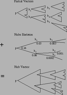
An intuitive view of the encoding and construction suggested by the Hubs
Equation (9) is shown in Figure 1.
Figure 1:
Intuitive view of the construction of hub vectors from
partial vectors and the hubs skeleton.
|
At the top, each partial vector
 , including
, is depicted as a notched triangle labeled at the tip.
The triangle can be thought of as representing paths starting at ,
although, more accurately, it represents the distribution of importance
scores computed based on the paths, as discussed in Section
4.1. A notch in the triangle shows where the computation of
a partial vector ``stopped'' at another hub page. At the center, a part
of the hubs skeleton is depicted as a tree so the ``assembly'' of
the hub vector can be visualized. The hub vector is constructed by logically
assembling the partial vectors using the corresponding weights in the hubs
skeleton, as shown at the bottom.
, including
, is depicted as a notched triangle labeled at the tip.
The triangle can be thought of as representing paths starting at ,
although, more accurately, it represents the distribution of importance
scores computed based on the paths, as discussed in Section
4.1. A notch in the triangle shows where the computation of
a partial vector ``stopped'' at another hub page. At the center, a part
of the hubs skeleton is depicted as a tree so the ``assembly'' of
the hub vector can be visualized. The hub vector is constructed by logically
assembling the partial vectors using the corresponding weights in the hubs
skeleton, as shown at the bottom.
4.4 Discussion
4.4.1 Summary
In summary, hub vectors are building blocks for PPV's corresponding to
preference vectors based on hub pages. Partial vectors, together with the
hubs skeleton, are building blocks for hub vectors. Transitively, partial
vectors and the hubs skeleton are building blocks for PPV's: they can be
used to construct PPV's without first materializing hub vectors as an
intermediate step (Section 5.4). Note that for
preference vectors based on multiple hub pages, constructing the
corresponding PPV from partial vectors directly can result in significant
savings versus constructing from hub vectors, since partial vectors are
shared across multiple hub vectors.
4.4.2 Choice of
So far we have made no assumptions about the set of hub pages . Not
surprisingly, the choice of hub pages can have a significant impact on
performance, depending on the location of hub pages within the overall graph
structure. In particular, the size of partial vectors is smaller when pages
in have higher PageRank, since high-PageRank pages are on average close
to other pages in terms of inverse P-distance (Section
4.1), and the size of the partial vectors is related to the
inverse P-distance between hub pages and other pages according to the Hubs
Theorem. Our intuition is that high-PageRank pages are generally more
interesting for personalization anyway, but in cases where the intended hub
pages do not have high PageRank, it may be beneficial to include some
high-PageRank pages in to improve performance. We ran experiments
confirming that the size of partial vectors is much smaller using
high-PageRank pages as hubs than using random pages.
4.4.3 Web Skeleton
The techniques used in the construction of hub vectors can be extended to
enable at least approximate personalization on arbitrary preference vectors
that are not necessarily based on . Suppose we want to personalize on a
page  . The Hubs Equation can be used to construct
from partial vectors, given that we have computed . As discussed in
Section 4.3, the cost of computing and storing
is orders of magnitude less than . Though is
only an approximation to , it may still capture significant
personalization information for a properly-chosen hub set , as
can be thought of as a ``projection'' of onto .
For example, if contains pages from Open Directory,
can capture information about the broad topic of . Exploring the
utility of the web skeleton
. The Hubs Equation can be used to construct
from partial vectors, given that we have computed . As discussed in
Section 4.3, the cost of computing and storing
is orders of magnitude less than . Though is
only an approximation to , it may still capture significant
personalization information for a properly-chosen hub set , as
can be thought of as a ``projection'' of onto .
For example, if contains pages from Open Directory,
can capture information about the broad topic of . Exploring the
utility of the web skeleton
 is an area
of future work.
is an area
of future work.
5. Computation
In Section 4 we presented a way to construct hub
vectors from partial vectors
, for , and
the hubs skeleton
. We also discussed the web
skeleton
. Computing these partial
quantities naively using a fixed-point iteration [11] for each
would scale poorly with the number of hub pages. Here we present scalable
algorithms that compute these quantities efficiently by using dynamic
programming to leverage the interrelationships among them. We also show how
PPV's can be constructed from partial vectors and the hubs skeleton at query
time. All of our algorithms have the property that they can be stopped at
any time (e.g., when resources are depleted), so that the current ``best
results'' can be used as an approximation, or the computation can be resumed
later for increased precision if resources permit.
We begin in Section 5.1 by presenting a
theorem underlying all of the algorithms presented (as well as the
connection between PageRank and inverse P-distance, as shown in the full
version [7]). In Section 5.2, we
present three algorithms, based on this theorem, for computing general basis
vectors. The algorithms in Section 5.2 are not meant
to be deployed, but are used as foundations for the algorithms in Section
5.3 for computing partial quantities. Section
5.4 discusses the construction of PPV's from
partial vectors and the hubs skeleton.
5.1 Decomposition Theorem
Recall the random surfer model of Section 1, instantiated
for preference vector
 (for page 's view of the web).
At each step, a surfer
(for page 's view of the web).
At each step, a surfer  teleports to page with some probability .
If is at , then at the next step, with probability will be
at a random out-neighbor of . That is, a fraction
teleports to page with some probability .
If is at , then at the next step, with probability will be
at a random out-neighbor of . That is, a fraction
 of the time, surfer will be at any given out-neighbor of one step
after teleporting to . This behavior is strikingly similar to the model
instantiated for preference vector
of the time, surfer will be at any given out-neighbor of one step
after teleporting to . This behavior is strikingly similar to the model
instantiated for preference vector
 , where surfers teleport directly to each
 with equal probability
 . The similarity is
formalized by the following theorem.
. The similarity is
formalized by the following theorem.
Theorem 3 (Decomposition)
For any ,
 |
(10) |
The Decomposition Theorem says that the basis vector
for is an average of the basis vectors
 for its
out-neighbors, plus a compensation factor
for its
out-neighbors, plus a compensation factor  . The proof is in the
full version [7].
. The proof is in the
full version [7].
The Decomposition Theorem gives another way to think about PPV's. It says
that 's view of the web () is the average of the views of its
out-neighbors, but with extra importance given to itself. That is, pages
important in 's view are either itself, or pages important in the
view of 's out-neighbors, which are themselves ``endorsed'' by . In
fact, this recursive intuition yields an equivalent way of formalizing
personalized PageRank scoring: basis vectors can be defined as vectors
satisfying the Decomposition Theorem.
While the Decomposition Theorem identifies relationships among basis
vectors, a division of the computation of a basis vector into
related subproblems for dynamic programming is not inherent in the
relationships. For example, it is possible to compute some basis vectors
first and then to compute the rest using the former as solved subproblems.
However, the presence of cycles in the graph makes this approach
ineffective. Instead, our approach is to consider as a subproblem the
computation of a vector to less precision. For example, having computed
to a certain precision, we can use the Decomposition
Theorem to combine the
's to compute to greater
precision. This approach has the advantage that precision needs not be fixed
in advance: the process can be stopped at any time for the current best
answer.
5.2 Algorithms for Computing Basis Vectors
We present three algorithms in the general context of computing full basis
vectors. These algorithms are presented primarily to develop our algorithms
for computing partial quantities, presented in Section
5.3. All three algorithms are iterative
fixed-point computations that maintain a set of intermediate results
![$(\bm{D_k[*], E_k[*]})$](img123.png) . For each ,
. For each , ![$\bm{D_k[p]}$](img124.png) is a
lower-approximation of on iteration , i.e.,
is a
lower-approximation of on iteration , i.e.,
 \leq
r_p(q)$](img125.png) for all . We build solutions (
for all . We build solutions (
 ) that are successively better approximations to , and
simultaneously compute the error components
) that are successively better approximations to , and
simultaneously compute the error components ![$\bm{E_k[p]}$](img127.png) , where
is the ``projection'' of the vector
, where
is the ``projection'' of the vector
![$(\bm{r_p} -
\bm{D_k[p]})$](img128.png) onto the (actual) basis vectors. That is, we maintain the
invariant that for all
onto the (actual) basis vectors. That is, we maintain the
invariant that for all  and all ,
![\begin{displaymath}
\bm{D_k[p]} + \sum_{q \in V}{E_k[p](q) \bm{r_q}} = \bm{r_p}
\end{displaymath}](img130.png) |
(11) |
Thus, is a lower-approximation of with error
We begin with
![$\bm{D_0[p]} = \bm{0}$](img132.png) and
and
![$\bm{E_0[p]} = \bm{x_p}$](img133.png) , so that logically, the approximation is initially
, so that logically, the approximation is initially
 and the error is . To store and
efficiently, we can represent them in an implementation as a
list of their nonzero entries. While all three algorithms have in common the
use of these intermediate results, they differ in how they use the
Decomposition Theorem to refine intermediate results on successive
iterations.
and the error is . To store and
efficiently, we can represent them in an implementation as a
list of their nonzero entries. While all three algorithms have in common the
use of these intermediate results, they differ in how they use the
Decomposition Theorem to refine intermediate results on successive
iterations.
It is important to note that the algorithms presented in this section and
their derivatives in Section 5.3 compute vectors
to arbitrary precision; they are not approximations. In practice, the
precision desired may vary depending on the application. Our focus is on
algorithms that are efficient and scalable with the number of hub vectors,
regardless of the precision to which vectors are computed.
5.2.1 Basic Dynamic Programming Algorithm
In the basic dynamic programming algorithm, a new basis vector for
each page is computed on each iteration using the vectors computed for
's out-neighbors on the previous iteration, via the Decomposition
Theorem. On iteration , we derive
![$(\bm{D_{k+1}[p]}, \bm{E_{k+1}[p]})$](img135.png) from
from
![$(\bm{D_k[p]}, \bm{E_k[p]})$](img136.png) using the equations:
using the equations:
A proof of the algorithm's correctness is given in the full version
[7], where the error ![$\vert\bm{E_k[p]}\vert$](img142.png) is shown to be reduced
by a factor of on each iteration.
is shown to be reduced
by a factor of on each iteration.
Note that although the ![$\bm{E_k[*]}$](img143.png) values help us to see the correctness
of the algorithm, they are not used here in the computation of
values help us to see the correctness
of the algorithm, they are not used here in the computation of ![$\bm{D_k[*]}$](img144.png) and can be omitted in an implementation (although they will be used to
compute partial quantities in Section 5.3). The
sizes of and grow with the number of iterations,
and in the limit they can be up to the size of , which is the
number of pages reachable from . Intermediate scores
and can be omitted in an implementation (although they will be used to
compute partial quantities in Section 5.3). The
sizes of and grow with the number of iterations,
and in the limit they can be up to the size of , which is the
number of pages reachable from . Intermediate scores
![$(\bm{D_k[*]},
\bm{E_k[*]})$](img145.png) will likely be much larger than available main memory, and in
an implementation
could be read off disk and
will likely be much larger than available main memory, and in
an implementation
could be read off disk and
![$(\bm{D_{k+1}[*]}, \bm{E_{k+1}[*]})$](img146.png) written to disk on each iteration. When
the data for one iteration has been computed, data from the previous
iteration may be deleted. Specific details of our implementation are
discussed in Section 6.
written to disk on each iteration. When
the data for one iteration has been computed, data from the previous
iteration may be deleted. Specific details of our implementation are
discussed in Section 6.
5.2.2 Selective Expansion Algorithm
The selective expansion algorithm is essentially a version of the
naive algorithm that can readily be modified to compute partial vectors, as
we will see in Section 5.3.1.
We derive
![$(\bm{D_{k+1}[p], E_{k+1}[p]})$](img147.png) by ``distributing'' the error at
each page (that is,
by ``distributing'' the error at
each page (that is, $](img148.png) ) to its out-neighbors via the
Decomposition Theorem. Precisely, we compute results on iteration- using
the equations:
) to its out-neighbors via the
Decomposition Theorem. Precisely, we compute results on iteration- using
the equations:
for a subset
 . If
. If  for all , then the
error is reduced by a factor of on each iteration, as in the basic
dynamic programming algorithm. However, it is often useful to choose a
selected subset of as
for all , then the
error is reduced by a factor of on each iteration, as in the basic
dynamic programming algorithm. However, it is often useful to choose a
selected subset of as  . For example, if contains the
 pages for which the error is highest, then this
top- scheme limits the number of expansions and delays the growth
in size of the intermediate results while still reducing much of the error.
In Section 5.3.1, we will compute the hub vectors by
choosing
pages for which the error is highest, then this
top- scheme limits the number of expansions and delays the growth
in size of the intermediate results while still reducing much of the error.
In Section 5.3.1, we will compute the hub vectors by
choosing  . The correctness of selective expansion is proven in
the full version [7].
. The correctness of selective expansion is proven in
the full version [7].
5.2.3 Repeated Squaring Algorithm
The repeated squaring algorithm is similar to the selective expansion
algorithm, except that instead of extending
one step using equations (14) and
(15), we compute what are essentially
iteration- results using the equations
where
. For now we can assume that for all
; we will set to compute the hubs skeleton in Section
5.3.2. The correctness of these equations is proven in the
full version [7], where it is shown that repeated squaring
reduces the error much faster than the basic dynamic programming or
selective expansion algorithms. If , the error is squared on
each iteration, as equation (17) reduces to:
![\begin{displaymath}
\bm{E_{2k}[p]} = \sum_{q \in V}{E_k[p](q)\bm{E_k[q]}}
\end{displaymath}](img160.png) |
(18) |
As an alternative to taking , we can also use the top- scheme
of Section 5.2.2.
Note that while all three algorithms presented can be used to compute the
set of all basis vectors, they differ in their requirements on the
computation of other vectors when computing : the basic dynamic
programming algorithm requires the vectors of out-neighbors of to be
computed as well, repeated squaring requires results
![$(\bm{D_k[q], E_k[q]})$](img161.png) to be computed for such that
to be computed for such that  > 0$](img162.png) , and selective expansion
computes independently.
, and selective expansion
computes independently.
5.3 Computing Partial Quantities
In Section 5.2 we presented iterative algorithms for
computing full basis vectors to arbitrary precision. Here we present
modifications to these algorithms to compute the partial quantities:

- Partial vectors
, .
-
- The hubs skeleton
(which can be computed more
efficiently by itself than as part of the entire web skeleton).
-
- The web skeleton
.
Each partial quantity can be computed in time no greater than its size,
which is far less than the size of the hub vectors.
5.3.1 Partial Vectors
Partial vectors can be computed using a simple specialization of the
selective expansion algorithm (Section
5.2.2): we take  and
and
 for
for  , for all . That is, we never ``expand'' hub
pages after the first step, so tours passing through a hub page are
never considered. Under this choice of ,
, for all . That is, we never ``expand'' hub
pages after the first step, so tours passing through a hub page are
never considered. Under this choice of ,
![$\bm{D_k[p]} + c
\bm{E_k[p]}$](img167.png) converges to
for all . Of
course, only the intermediate results
for should be computed. A proof is presented in the full version
[7].
converges to
for all . Of
course, only the intermediate results
for should be computed. A proof is presented in the full version
[7].
This algorithm makes it clear why using high-PageRank pages as hub pages
improves performance: from a page we expect to reach a high-PageRank
page sooner than a random page, so the expansion from will stop
sooner and result in a shorter partial vector.
5.3.2 Hubs Skeleton
While the hubs skeleton is a subset of the complete web skeleton and can be
computed as such using the technique to be presented in Section
5.3.3, it can be computed much faster by itself if we are
not interested in the entire web skeleton, or if higher precision is desired
for the hubs skeleton than can be computed for the entire web skeleton.
We use a specialization of the repeated squaring algorithm (Section
5.2.3) to compute the hubs skeleton, using
the intermediate results from the computation of partial vectors. Suppose
, for  , have been computed by the
algorithm of Section 5.3.1, so that
, have been computed by the
algorithm of Section 5.3.1, so that
 < \epsilon$](img169.png) , for some error
, for some error  . We apply the repeated
squaring algorithm on these results using for all successive
iterations. As shown in the full version [7], after
iterations of repeated squaring, the total error
. We apply the repeated
squaring algorithm on these results using for all successive
iterations. As shown in the full version [7], after
iterations of repeated squaring, the total error ![$\vert\bm{E_i[p]}\vert$](img171.png) is bounded
by
is bounded
by
 . Thus, by varying and , can
be computed to arbitrary precision.
. Thus, by varying and , can
be computed to arbitrary precision.
Notice that only the intermediate results
![$(\bm{D_k[h], E_k[h]})$](img173.png) for are ever needed to update scores for , and of the former,
only the entries
for are ever needed to update scores for , and of the former,
only the entries
, E_k[h](q)$](img174.png) , for
, for  , are used to compute
$](img176.png) . Since we are only interested in the hub scores , we
can simply drop all non-hub entries from the intermediate results. The
running time and storage would then depend only on the size of and
not on the length of the entire hub vectors . If the restricted
intermediate results fit in main memory, it is possible to defer the
computation of the hubs skeleton to query time.
. Since we are only interested in the hub scores , we
can simply drop all non-hub entries from the intermediate results. The
running time and storage would then depend only on the size of and
not on the length of the entire hub vectors . If the restricted
intermediate results fit in main memory, it is possible to defer the
computation of the hubs skeleton to query time.
5.3.3 Web Skeleton
To compute the entire web skeleton, we modify the basic dynamic programming
algorithm (Section 5.2.1) to compute only the hub scores
, with corresponding savings in time and memory usage. We restrict
the computation by eliminating entries  from the intermediate
results
, similar to the technique used in
computing the hubs skeleton.
from the intermediate
results
, similar to the technique used in
computing the hubs skeleton.
The justification for this modification is that the hub score
$](img178.png) is affected only by the hub scores
is affected only by the hub scores $](img179.png) of the
previous iteration, so that in the modified algorithm is
equal to that in the basic algorithm. Since is likely to be orders of
magnitude less than , the size of the intermediate results is reduced
significantly.
of the
previous iteration, so that in the modified algorithm is
equal to that in the basic algorithm. Since is likely to be orders of
magnitude less than , the size of the intermediate results is reduced
significantly.
5.4 Construction of PPV's
Finally, let us see how a PPV for preference vector can be
constructed directly from partial vectors and the hubs skeleton using the
Hubs Equation. (Construction of a single hub vector is a specialization of
the algorithm outlined here.) Let
 be a preference vector, where
  for
for
 . Let
. Let
 , and let
 |
(19) |
which can be computed from the hubs skeleton. Then the PPV for
can be constructed as
![\begin{displaymath}
\bm{v} = \sum_{i=1}^{z} \alpha_i (\bm{r_{p_i}-r_{p_i}^...
... r_u(h) > 0}}
r_u(h)\left[(\bm{r_h-r_h^H})-c\bm{x_h}\right]
\end{displaymath}](img185.png) |
(20) |
Both the terms
 and
are partial
vectors, which we assume have been precomputed. The term
represents a simple subtraction from
. If
and
are partial
vectors, which we assume have been precomputed. The term
represents a simple subtraction from
. If  , then
 represents a full construction of .
However, for some applications, it may suffice to use only parts of the hubs
skeleton to compute to less precision. For example, we can take
represents a full construction of .
However, for some applications, it may suffice to use only parts of the hubs
skeleton to compute to less precision. For example, we can take
 to be the hubs for which
  is highest. Experimentation
with this scheme is discussed in Section 6.3.
Alternatively, the result can be improved incrementally (e.g., as time
permits) by using a small subset each time and accumulating the results.
is highest. Experimentation
with this scheme is discussed in Section 6.3.
Alternatively, the result can be improved incrementally (e.g., as time
permits) by using a small subset each time and accumulating the results.
6. Experiments
We performed experiments using real web data from Stanford's WebBase
[6], a crawl of the web containing 120 million pages. Since the
iterative computation of PageRank is unaffected by leaf pages (i.e.,
those with no out-neighbors), they can be removed from the graph and added
back in after the computation [11]. After removing leaf pages, the
graph consisted of 80 million pages
Both the web graph and the intermediate results
were
too large to fit in main memory, and a partitioning strategy, based on that
presented in [4], was used to divide the computation into
portions that can be carried out in memory. Specifically, the set of pages
was partitioned into arbitrary sets
 of equal size
(
of equal size
( in our experiments). The web graph, represented as an edge-list
, is partitioned into chunks
in our experiments). The web graph, represented as an edge-list
, is partitioned into chunks  (
(
 ), where
contains all edges
for which
), where
contains all edges
for which  .
Intermediate results and were represented
together as a list
.
Intermediate results and were represented
together as a list
![$\bm{L_k[p]} = \langle (q_1, d_1, e_1), (q_2, d_2, e_2),
\dots \rangle$](img196.png) where
where
 = d_z$](img197.png) and
and
 = e_z$](img198.png) , for
, for
 . Only pages
  for which either
  or
or  were
included. The set of intermediate results
were
included. The set of intermediate results ![$\bm{L_k[*]}$](img203.png) was partitioned into
was partitioned into
 chunks
![$\bm{L_k^{i,j}[*]}$](img205.png) , so that
, so that
![$\bm{L_k^{i,j}[p]}$](img206.png) contains
triples
contains
triples
 of
of ![$\bm{L_k[p]}$](img208.png) for which and
for which and  . In each of the algorithms for computing partial quantities, only
a single column
. In each of the algorithms for computing partial quantities, only
a single column
![$\bm{L_k^{*,j}[*]}$](img210.png) was kept in memory at any one time, and
part of the next-iteration results
was kept in memory at any one time, and
part of the next-iteration results
![$\bm{L_{k+1}[*]}$](img211.png) were computed by
successively reading in individual blocks of the graph or intermediate
results as appropriate. Each iteration requires only one linear scan of the
intermediate results and web graph, except for repeated squaring, which does
not use the web graph explicitly.
were computed by
successively reading in individual blocks of the graph or intermediate
results as appropriate. Each iteration requires only one linear scan of the
intermediate results and web graph, except for repeated squaring, which does
not use the web graph explicitly.
6.1 Computing Partial Vectors
For comparison, we computed both (full) hub vectors and partial vectors for
various sizes of , using the selective expansion algorithm with (full hub vectors) and
(partial vectors). As discussed
in Section 4.4.2, we found the partial vectors approach
to be much more effective when contains high-PageRank pages rather than
random pages. In our experiments ranged from the top  to top
 pages with the highest PageRank. The constant was set to
 .
.
To evaluate the performance and scalability of our strategy independently of
implementation and platform, we focus on the size of the results rather than
computation time, which is linear in the size of the results. Because of the
number of trials we had to perform and limitations on resources, we computed
results only up to 6 iterations, for up to .
Figure 2:
Average Vector Size vs. Number of Hubs
|
Figure 2 plots the average size of (full) hub vectors and
partial vectors (recall that size is the number of nonzero entries), as
computed after 6 iterations of the selective expansion algorithm, which for
computing full hub vectors is equivalent to the basic dynamic programming
algorithm. Note that the x-axis plots in logarithmic scale.
Experiments were run using a 1.4 gigahertz CPU on a machine with 3.5
gigabytes of memory. For  , the computation of full hub vectors
took about
, the computation of full hub vectors
took about  seconds per vector, and about
  seconds for each
partial vector. We were unable to compute full hub vectors for
seconds for each
partial vector. We were unable to compute full hub vectors for
 due to the time required, although the average vector size is
expected not to vary significantly with for full hub vectors. In
Figure 2 we see that the reduction in size from using our
technique becomes more significant as increases, suggesting that our
technique scales well with .
due to the time required, although the average vector size is
expected not to vary significantly with for full hub vectors. In
Figure 2 we see that the reduction in size from using our
technique becomes more significant as increases, suggesting that our
technique scales well with .
6.2 Computing the Hubs Skeleton
We computed the hubs skeleton for  by running the selective
expansion algorithm for
by running the selective
expansion algorithm for  iterations using , and then running
the repeated squaring algorithm for
iterations using , and then running
the repeated squaring algorithm for  iterations (Section
5.3.2), where is chosen to be the top 50 entries
under the top- scheme (Section 5.2.2).
The average size of the hubs skeleton is
iterations (Section
5.3.2), where is chosen to be the top 50 entries
under the top- scheme (Section 5.2.2).
The average size of the hubs skeleton is  entries. Each iteration of
the repeated squaring algorithm took about an hour, a cost that depends only
on and is constant with respect to the precision to which the partial
vectors are computed.
entries. Each iteration of
the repeated squaring algorithm took about an hour, a cost that depends only
on and is constant with respect to the precision to which the partial
vectors are computed.
6.3 Constructing Hub Vectors from Partial Vectors
Next we measured the construction of (full) hub vectors from partial vectors
and the hubs skeleton. Note that in practice we may construct PPV's directly
from partial vectors, as discussed in Section 5.4.
However, performance of the construction would depend heavily on the user's
preference vector. We consider hub vector computation because it better
measures the performance benefits of our partial vectors approach.
As suggested in Section 4.3, the precision of the
hub vectors constructed from partial vectors can be varied at query time
according to application and performance demands. That is, instead of using
the entire set in the construction of , we can use only
the highest entries, for  .
.
Figure 3:
Construction Time and Size vs. Hubs Skeleton Portion ()
|
Figure 3 plots the average size and time required to construct a
full hub vector from partial vectors in memory versus , for . Results are averaged over  randomly-chosen hub vectors. Note
that the x-axis is in logarithmic scale.
randomly-chosen hub vectors. Note
that the x-axis is in logarithmic scale.
Recall from Section 6.1 that the partial vectors from
which the hubs vector is constructed were computed using 6 iterations,
limiting the precision. Thus, the error values in Figure 3 are
roughly  (ranging from
  for
for  to
to  for
for  ). Nonetheless, this error is much smaller than that of the
iteration- full hub vectors computed in Section 6.1,
which have error
). Nonetheless, this error is much smaller than that of the
iteration- full hub vectors computed in Section 6.1,
which have error
 . Note, however, that the size of a vector
is a better indicator of precision than the magnitude, since we are usually
most interested in the number of pages with nonzero entries in the
distribution vector. An iteration-6 full hub vector (from Section
6.1) for page contains nonzero entries for pages at
most 6 links away from ,
. Note, however, that the size of a vector
is a better indicator of precision than the magnitude, since we are usually
most interested in the number of pages with nonzero entries in the
distribution vector. An iteration-6 full hub vector (from Section
6.1) for page contains nonzero entries for pages at
most 6 links away from ,  pages on average. In contrast, from
Figure 3 we see that a hub vector containing 14 million nonzero
entries can be constructed from partial vectors in 6 seconds.
pages on average. In contrast, from
Figure 3 we see that a hub vector containing 14 million nonzero
entries can be constructed from partial vectors in 6 seconds.
7. Related Work
The use of personalized PageRank to enable personalized web search was first
proposed in [11], where it was suggested as a modification of the
global PageRank algorithm, which computes a universal notion of importance.
The computation of (personalized) PageRank scores was not addressed beyond
the naive algorithm.
In [5], personalized PageRank scores were used to enable
``topic-sensitive'' web search. Specifically, precomputed hub vectors
corresponding to broad categories in Open Directory were used to bias
importance scores, where the vectors and weights were selected according to
the text query. Experiments in [5] concluded that the use of
personalized PageRank scores can improve web search, but the number of hub
vectors used was limited to 16 due to the computational requirements, which
were not addressed in that work. Scaling the number of hub pages beyond 16
for finer-grained personalization is a direct application of our work.
Another technique for computing web-page importance, HITS, was
presented in [9]. In HITS, an iterative computation
similar in spirit to PageRank is applied at query time on a subgraph
consisting of pages matching a text query and those ``nearby''.
Personalizing based on user-specified web pages (and their linkage structure
in the web graph) is not addressed by HITS. Moreover, the number of pages in
the subgraphs used by HITS (order of thousands) is much smaller than that we
consider in this paper (order of millions), and the computation from scratch
at query time makes the HITS approach difficult to scale.
Another algorithm that uses query-dependent importance scores to improve
upon a global version of importance was presented in [12]. Like
HITS, it first restricts the computation to a subgraph derived from text
matching. (Personalizing based on user-specified web pages is not
addressed.) Unlike HITS, [12] suggested that importance scores be
precomputed offline for every possible text query, but the enormous number
of possibilities makes this approach difficult to scale.
The concept of using ``hub nodes'' in a graph to enable partial computation
of solutions to the shortest-path problem was used in [3] in
the context of database search. That work deals with searches within
databases, and on a scale far smaller than that of the web.
Some system aspects of (global) PageRank computation were addressed in
[4]. The disk-based data-partitioning strategy used in the
implementation of our algorithm is adopted from that presented therein.
Finally, the concept of inverse P-distance used in this paper is based on
the concept of expected- distance introduced in [8], where it
was presented as an intuitive model for a similarity measure in graph
structures.
8. Summary
We have addressed the problem of scaling personalized web search:
- We started by identifying a linear relationship that allows
personalized PageRank vectors to be expressed as a linear combination of
basis vectors. Personalized vectors corresponding to arbitrary
preference sets drawn from a hub set can be constructed quickly
from the set of precomputed basis hub vectors, one for each hub .
- We laid the mathematical foundations for constructing hub vectors
efficiently by relating personalized PageRank scores to inverse
P-distances, an intuitive notion of distance in arbitrary directed
graphs. We used this notion of distance to identify interrelationships
among basis vectors.
- We presented a method of encoding hub vectors as partial
vectors and the hubs skeleton. Redundancy is minimized under
this representation: each partial vector for a hub page represents the
part of 's hub vector unique to itself, while the skeleton specifies
how partial vectors are assembled into full vectors.
- We presented algorithms for computing basis vectors, and showed how
they can be modified to compute partial vectors and the hubs skeleton
efficiently.
- We ran experiments on real web data showing the effectiveness of our
approach. Results showed that our strategy results in significant resource
reduction over full vectors, and scales well with , the degree of
personalization.
The authors thank Taher Haveliwala for many useful discussions and extensive
help with implementation.
- 1
-
http://www.google.com.
- 2
-
http://dmoz.org.
- 3
-
R. Goldman, N. Shivakumar, S. Venkatasubramanian, and H. Garcia-Molina.
Proximity search in databases.
In Proceedings of the Twenty-Fourth International Conference on
Very Large Databases, New York, New York, Aug. 1998.
- 4
-
T. H. Haveliwala.
Efficient computation of PageRank.
Technical report, Stanford University Database Group, 1999.
http://dbpubs.stanford.edu/pub/1999-31.
- 5
-
T. H. Haveliwala.
Topic-sensitive PageRank.
In Proceedings of the Eleventh International World Wide Web
Conference, Honolulu, Hawaii, May 2002.
- 6
-
J. Hirai, S. Raghavan, A. Paepcke, and H. Garcia-Molina.
WebBase: A repository of web pages.
In Proceedings of the Ninth International World Wide Web
Conference, Amsterdam, Netherlands, May 2000.
http://www-diglib.stanford.edu/~testbed/doc2/WebBase/.
- 7
-
G. Jeh and J. Widom.
Scaling personalized web search.
Technical report, Stanford University Database Group, 2002.
http://dbpubs.stanford.edu/pub/2002-12.
- 8
-
G. Jeh and J. Widom.
SimRank: A measure of structural-context similarity.
In Proceedings of the Eighth ACM SIGKDD International
Conference on Knowledge Discovery and Data Mining, Edmonton, Alberta,
Canada, July 2002.
- 9
-
J. M. Kleinberg.
Authoritative sources in a hyperlinked environment.
In Proceedings of the Ninth Annual ACM-SIAM Symposium on
Discrete Algorithms, San Francisco, California, Jan. 1998.
- 10
-
R. Motwani and P. Raghavan.
Randomized Algorithms.
Cambridge University Press, United Kingdom, 1995.
- 11
-
L. Page, S. Brin, R. Motwani, and T. Winograd.
The PageRank citation ranking: Bringing order to the Web.
Technical report, Stanford University Database Group, 1998.
http://citeseer.nj.nec.com/368196.html.
- 12
-
M. Richardson and P. Domingos.
The intelligent surfer: Probabilistic combination of link and content
information in PageRank.
In Proceedings of Advances in Neural Information Processing
Systems 14, Cambridge, Massachusetts, Dec. 2002.
This work was supported by
the National Science Foundation under grant IIS-9817799. This is an
abbreviated version of the full paper that omits appendices. The full
version is available on the web at
http://dbpubs.stanford.edu/pub/2002-12.
Copyright is held by the author/owner(s).
WWW2003, May 20-24, 2003, Budapest, Hungary.
ACM 1-58113-449-5/02/0005
Footnotes
- [footnote 1]
- Specifically, corresponds to the
steady-state distribution of an ergodic, aperiodic
Markov chain.
- [footnote 2]
- More precisely, the transformation from personalization
vectors to their corresponding solution vectors is
linear.
- [footnote 3]
- Note that while the mathematics and computation
strategies in this paper are presented in the specific context of the web
graph, they are general graph-theoretical results that may be applicable
in other scenarios involving stochastic processes, of which PageRank is one
example.
- [footnote 4]
- The
definition here of inverse P-distance differs slightly from the concept of
expected- distance in [8], where tours are not allowed to
visit multiple times. Note that general expected- distances have the
form
![$\sum_{t}{P[t]f(l(t))}$](img77.png) ; in our definition,
; in our definition,
 .
.
This document was generated using the
LaTeX2HTML translator Version 2002-2 (1.70)
\bm{r_q}} \right\vert =
\left\vert\bm{E_k[p]}\right\vert\end{displaymath}](img131.png)
![$\displaystyle \frac{1-c}{\vert O(a)\vert} \sum\limits_{i=1}^{\vert O(p)\vert}{\bm{D_{k}[O_i(p)]}} + c\bm{x_p}$](img139.png)
![$\displaystyle \frac{1-c}{\vert O(a)\vert} \sum\limits_{i=1}^{\vert O(p)\vert}{\bm{E_{k}[O_i(p)]}}$](img141.png)
![$\displaystyle \bm{D_k[p]} + \sum_{q \in Q_k(p)}{c \cdot E_k[p](q)\bm{x_q}}$](img149.png)
![$\displaystyle \bm{E_k[p]} - \sum_{q \in Q_k(p)}{E_k[p](q)\bm{x_q}} +
\sum_{q \i...
...{1-c}{\vert O(q)\vert}\sum_{i = 1}^{\vert O(q)\vert}
{E_k[p](q)\bm{x_{O_i(q)}}}$](img150.png)
![$\displaystyle \bm{D_k[p]} + \sum_{q \in Q_k(p)}{E_k[p](q)\bm{D_k[q]}}$](img157.png)
![$\displaystyle \bm{E_k[p]} - \sum_{q \in Q_k(p)}{E_k[p](q)\bm{x_q}} +
\sum_{q \in Q_k(p)}{E_k[p](q)\bm{E_k[q]}}$](img159.png)
![\scalebox{0.42}[0.4]{\includegraphics{numHubs}}](img215.png)
![\scalebox{0.42}[0.4]{\includegraphics{m}}](img225.png)