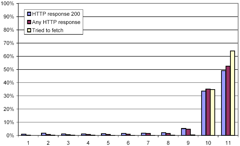
Figure 1: Successfully downloaded versions of URLs
The searchable web and the search engines which survey it have become indispensable tools for information discovery. From academic researchers to elementary-school students, from cancer patients to pensioners, from local high-school football fans to international travelers, the indexed content of the web is becoming the primary research tool for many. With hundreds of millions of people relying on these tools, one is led to ask if the tools provide useful, up-to-date results. Ideally, one would like the entire index of a search engine to be fresh, that is, to contain the most up-to-date version of a web page. The Google search engine attempts to maintain a fresh index by crawling over 3 billion pages once a month [7], with more frequent crawls of hand-selected sites that are known to change more often. In addition, it offers access to cached copies of pages, to obviate problems arising some of the crawled URLs being out-of-date or having disappeared entirely.
To improve the freshness of results returned by search engines and allow them to spend more of their efforts crawling and indexing pages which have changed, it is interesting and important to answer some questions about the dynamic nature of the web. How fast does the web change? Does most of the content remain unchanged once it has been authored, or are the documents being continuously updated? Do pages change a little or a lot? Is the extent of change correlated to any other property of the page? Do pages change and then change back? How consistent are mirrors and near-mirrors of pages? Questions like these are of great relevance to search engines, and more generally to any party trying to maintain an up-to-date view of the web, but they are also interesting in their own right, as they shed light on the evolution of a major sociological phenomenon: the largest collectively constructed information repository known to man.
In this paper, we attempt to answer some of these questions. We recount how we collected 151 million web pages eleven times over, retaining salient information including a feature vector of each page. We describe how we distilled the collected information about each URL into a summary record, tabulating the feature vectors. We sketch the framework we used to mine the distilled data for statistical information. We present the most interesting results of this data mining. Finally, we draw some conclusions and offer avenues of future work.
This paper expands on a study by Cho and Garcia-Molina [5]. The authors of that study downloaded 720,000 pages drawn from 270 "popular" web servers (not exceeding 3,000 pages per server) on a daily basis over the course of four months, and retained the MD5 checksum of the contents (including the HTML markup) of each page. This allowed them to determine if a document had changed, although it did not allow them to assess the degree of change. Among other things, they found that pages drawn from servers in the .com domain changed substantially faster than those in other domains, while pages in the .gov domain changed substantially slower. Overall, they found that about 40% of all web pages changed within a week, and that it took about 50 days for half of all pages to have changed. They also found that almost 25% of the pages in .com changed within a day, and that it took 11 days for half of all .com pages to have changed. By contrast, it took four months (the duration of their study) for half of the .gov pages to have changed.
Sun et al. [11] studied the efficacy of web anonymizers. As part of that study, they drew a set of 100,000 web pages from the Open Directory listing, and crawled each page twice, with the second retrieval immediately following the first one. Since they were interested in the information leakage of encrypted channels, they did not compare checksums of the returned pages; rather, they compared the lengths of the pages and the number and lengths of their embedded images and frames (which will appear to an eavesdropper as temporally closely spaced TCP packets). They found that 40% of pages changed signatures, and that 14% of pages changed by 30% or more, using a Jaccard-coefficient-based similarity metric akin to the one we use, but based on the size of a document including sizes of embedded images, not contents.
Douglis et al. [6] studied a web trace consisting of 950,000 entries (each entry representing a web access) collected over 17 days at the gateway between AT&T Labs-Research and the Internet. They recorded the "last-modified" timestamp transmitted by the web server (implicitly assuming that web servers transmit accurate information). In addition, they mined each page for items such as phone numbers using a domain-specific semantic analysis technique called "grinking", and measured the rate of change of these items. They found that according to the last-modified metric, 16.5% of the resources (including HTML pages as well as other content, such as images) that were accessed multiple times changed every time they were accessed. They also found that among the HTML pages that were accessed more than once, almost 60% experienced a change in HREF links, and over 50% of them experienced a change in IMG links.
Brewington and Cybenko built a web clipping service, which they leveraged to study the change rate of web pages [1]. They did so by recording the last-modified time stamp, the time of download, and various stylistic attributes (number of images, links, tables, etc) of each downloaded HTML page. Their service downloaded about 100,000 pages per day, selected based on their topical interest, recrawling no page more often than once every three days. They evaluated data collected between March and November 1999. For pages that were downloaded six times or more, 56% did not change at all over the duration of the study (according to the features they retained), while 4% changed every single time.
Our study differs from previous studies in several respects. First, it covers a roughly 200 times larger portion of the web (although the interval between revisits is seven times larger than, say, the one used by Cho and Garcia-Molina). Second, we used a different and more fine-grained similarity metric than any of the other studies, based on syntactic document sketches [4]. Third, we selected our pages based on a breadth-first crawl, which removed some of the bias inherent in the other studies (although breadth-first crawling is known to be biased towards pages with high PageRank [9]). Fourth and finally, we retained the full text of 0.1% of all downloaded pages, a sample set that is comparable in size to the set of pages summarized by other studies.
Our experiment can be divided into three phases: Collecting the data through repeated web crawls, distilling the data to make it amenable to analysis, and mining the distillate. This section describes each of the phases in more detail.
Between 26 Nov. 2002 and 5 Dec. 2002, we performed a large crawl ("crawl 1") that downloaded 151 million HTML pages as well as 62 million non-HTML pages, which we subsequently ignored. We then attempted to fetch each of these 151 million HTML pages ten more times over a span of ten weeks. Naturally, some of these pages became either temporarily or permanently unavailable. Moreover, we experienced a catastrophic disk failure during the third crawl, causing us to lose a quarter of the logs of that crawl. Figure 1 shows the distribution of successful downloads. As can be seen, we succeeded in downloading 49.2% of the pages all eleven times, and 33.6% ten times, leaving 17.2% of the pages that could only be downloaded nine times or fewer.
Figure 1: Successfully downloaded versions of URLs
Our hardware infrastructure consisted of a cluster of four Compaq DS20 servers, each one equipped with a 667 MHz Alpha processor, 4 GB of RAM, 648 GB of disk, and a fast Ethernet network connection. The machines were located at the Palo Alto Internet Exchange, a peering point for 12 Telcos and 20 major and about 130 minor ISPs.
We conducted these crawls using the Mercator web crawler [8]. Mercator is both fast and highly configurable, making it a suitable tool for our purposes.
We seeded crawl 1 with the Yahoo! home page. We restricted ourselves to content retrievable using HTTP, ignoring HTTPS, FTP, Gopher, and the like. Mercator crawled using its standard breadth-first search web traversal strategy, which is biased towards pages with high PageRank [9]. This crawl ran for 9 days, and downloaded a total of 6.4 TB of data. As said earlier, it logged the URLs of 151 million HTML pages that were successfully retrieved, i.e. that were returned with an HTTP status code of 200 and a content type of text/html.
We used these 151 million URLs to seed the following ten crawls. These crawls ran consecutively, starting on 5 Dec. 2002 and ending on 12 Feb. 2003. We disabled link extraction and HTTP redirections; in other words, we configured Mercator to fetch only the pages in its seed set. Every crawl slowed down by two orders of magnitude once it had processed all but a million or so seeds, because the remaining URLs all referred to web servers that were extremely slow to respond to us during that crawl, and because Mercator's politeness policies cause it to space out requests to the same host proportional to the delay of the previous response from that host. In order to keep the overall duration of each crawl within reasonable bounds, we terminated the crawls after this happened, typically on the sixth day of the crawl, and started the next crawl a week after the start of the preceding one.
For all eleven crawls, we provided Mercator with two new processing modules: a module that recorded a checksum and a fixed-size feature vector plus some ancillary data for each page, and a second module that selected 0.1% of all pages and saved them to disk.
We computed the feature vectors using a modified version of the document shingling technique due to Broder et al. [4], which uses a metric of document similarity based on syntactic properties of the document. This similarity metric is applicable to any kind of document that consists of an ordered sequence of discrete features. The following description assumes that the features are words, i.e. that a document is an ordered sequence of words. In order to compare two documents, we map each document into a set of k-word subsequences (groups of adjacent words or "shingles"), wrapping at the end of the document, so that every word in the document starts a shingle.
Two documents are considered to be identical if they map to the same set of shingles;1 they are considered to be similar if they map to similar sets of shingles. Quantitatively, the similarity of two documents is defined to be the number of distinct shingles appearing in both documents divided by the total number of distinct shingles. This means that two identical documents have similarity 1, while two documents that have no shingle in common have similarity 0.
Note that the value of k parameterizes how sensitive this metric is. Changing the word "kumquat" to "persimmon" in an n-word document (assuming that "kumquat" and "persimmon" occur nowhere else in the document) results in a similarity of [(n-k)/(n+k)] between the original and the modified document. This means that one should not choose k to be too large, lest even small changes result in low similarity. On the other hand, neither should one choose k to be too small. As an extreme example, setting k to 1 results in a comparison of the lexicon of two documents, making the metric completely insensitive to word ordering.
Our feature vector extraction module substitutes HTML markup by whitespace, and then segments the document into 5-word shingles, where each word is an uninterrupted sequence of alphanumeric characters. Next, it computes a 64-bit checksum of each shingle, using Rabin's fingerprinting algorithm [3,10]. We call these fingerprints the "pre-images". Next, the module applies 84 different (randomly selected but fixed thereafter) one-to-one functions to each pre-image. For each function, we retain the pre-image which results in the numerically smallest image. This results in a vector of 84 pre-images, which is the desired feature vector.
If the one-to-one functions are chosen randomly,2 then given the feature vectors of two documents, two corresponding elements of the vectors are identical with probability equal to the similarity of the documents.
The feature vector extraction module logs the feature vector of each document, together with a checksum of its raw content, the start time and the duration of its retrieval, the HTTP status code (or an error code indicating a TCP error or a robot exclusion), the document's length, the number of non-markup words, and the URL. If the document cannot be downloaded successfully or does not result in an HTML document,3 the module logs the URL and special values for everything else. URLs that were not downloaded because the crawl was terminated before it was complete are treated in a similar fashion.
The document sampling module saves those successfully downloaded documents whose URLs hash to 0 modulo 1000; in other words, it saves 0.1% of all downloaded documents (assuming we used a uniform hash function). The log contains the URL of each document as well as the entire HTTP response to each request, which includes the HTTP header as well as the document.
Crawling left us with 44 very large logs (produced by the eleven crawls on the four crawlers), each spanning multiple files, one per day. The logs totaled about 1,200 GB, whereas the sampled documents took up a mere 59 GB.
As they were, these logs were not suitable for analysis yet, because the URLs occurred in non-deterministic order in each log. One way to rectify this would be to perform a merge-sort of the logs based on their URL, in order to bring together the various occurrences of each URL. However, performing such a merge-sort on 1,200 GB of data is prohibitively expensive. To overcome this problem, we bucketized each of the logs, dividing its contents over 1,000 buckets, using the same URL-based hash function as in the document sampling module. This step produced 44,000 buckets (1,000 buckets per crawler per crawl). While this might appear to double the storage requirement, we could process an individual daily log file, and then move it to near-line storage. As a result of the bucketization, all the occurrences of a given URL appear in corresponding buckets across generations, and each bucket is less than 30 MB in size. This allowed us to then perform a fast in-memory sort of each bucket, using the URL as the key, and replacing the original bucket with a sorted one.
At the end of this process, the corresponding buckets of each generation all contained exactly the same set of URLs, in sorted order.
Finally, we merged the buckets across crawls, and distilled them in the process. We did so by iterating on all four machines over the 1,000 bucket classes, reading a record at a time from each of the eleven corresponding buckets, and writing a combined record to a distilled bucket. Each combined record contains the following information:
Note that the distilled record does not include the checksums or the pre-images of each document. These values are subsumed by the "supershingles", the bit-vectors, and the match counts.
Each of the six "supershingles" represents the concatenation of 14 adjacent pre-images. Due to the independence of the one-to-one functions used to select pre-images, if two documents have similarity p, each of their supershingles matches with probability p14. For two documents that are 95% similar, each supershingle matches its counterpart with probability 49%. Given that we retain six supershingles, there is a probability of almost 90% that at least two of the six supershingles will agree for documents that are 95% or more similar. Retaining the supershingles will be useful in the future, should we try to discover approximate mirrors [2] and investigate their update frequency.
The match count, when non-negative, indicates how many of the 84 pre-image pairs matched between the two documents. If the document fingerprint matches as well, the match count is set to 85. The match count is negative if either document was not downloaded successfully or contained no words at all (which caused the pre-images to have a default value); its value indicates which condition applied to which document, and whether the documents were identical (i.e. their checksums matched).
While the original logs were 1,200 GB in size, the distilled buckets consume only about 222 GB. Even so, it still takes about 10 hours to read the distilled logs. In order to conduct the statistical experiments we report on below (as well as a number of others which proved less informative), we needed to find a way to conduct each experiment considerably faster. We achieve this by running several experiments at once, thereby amortizing the cost of reading the logs over multiple experiments.
Using this approach, we were no longer limited by our computer's ability to read the logs, but rather by our ability to decide a priori which experiments would be interesting and relevant. Given the trial-and-error character of any data mining activity, we still had to do several passes over the data to construct all of the experiments described below.
We built an analyzer harness that reads through the distilled buckets one record at a time, expands each record into an easy-to-use format, and presents it to each of a set of analyzer modules. Once all buckets have been read, the harness invokes a "finish" method on each of the analyzers, causing them to write out any aggregate statistics they may have gathered. The analyzers as well as the harness are written in Java; the harness uses Java's dynamic class loading capabilities to load the analyzers at run-time.
Examples of the analyzers we wrote include:
Analyzers can be nested into higher-level analyzers. For example, it is possible to put a ChangeAnalyzer into a TopLevelDomainAnalyzer, producing a list of document change histograms, one for each top-level domain. This is again implemented using Java's dynamic class loading machinery. In order to keep the size of the output manageable, we also provide ways to limit the number of top-level domains considered (putting all unspecified domains into a catch-all category), to group numbers of unchanged pre-images into clusters, and the like.
For some of these higher-level analyzers, we need to aggregate multiple values (for example, the sizes of the eleven versions of a web page) into a single value, in order to decide what lower-level analyzer to invoke. We currently provide three different ways to aggregate values, namely minimum, maximum, and average. We plan to add support for mode, median, and geometric average.
Recall that during the data collection phase, we saved the full text of 0.1% of all successfully downloaded pages. We selected these pages based on a hash of the URL, using the same hash function as the bucketizer. In particular, we saved the full text of all pages that went into bucket 0. This enables us to use the analyzer framework to detect interesting patterns, to use a special analyzer (using higher-level analyzers around a "DumpURLAnalyzer") to get a listing of all URLs in bucket 0 that fit this pattern, and then to examine the full text of some of these documents.
We built some infrastructure to make this process easier. In particular, we prepend each file of sampled documents with an index of URLs and document offsets, which allows us to retrieve any page in constant time. Second, we implemented a web service that accepts a URL, a version number, and whether to return the HTTP header or the document, and returns the requested item for display in the browser. Third, we implemented another web service that accepts a list of analyses to run, executes them on a subset of the distilled buckets, and returns the results as a web page. We hope to make these services, as well as some of the distilled buckets, available to the research community.
The results presented in this section are derived from analyzing the 151 million distilled records in our collection, using the analyzer harness and many of the analyzers described above.
Figure 2 shows a histogram of document length, for all of the 1,482,416,213 documents that were successfully downloaded (i.e. that had an HTTP status code of 200), as well as broken out by a few selected top-level domains. The x-axis denotes the document size; a value of n means that the size of the document was below 2n bytes, but not below 2n-1 bytes (a value of 0 indicates that the document had length 0).
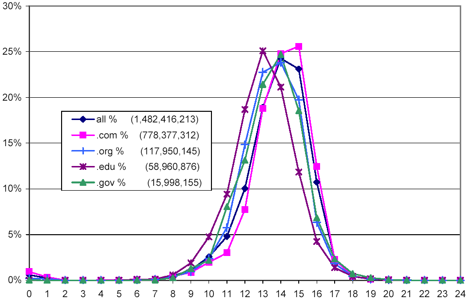
Figure 2: Distribution of documents lengths overall and for selected top-level domains.
The distribution we observed centers at 14 with standard deviation 1; 66.3% of all observed HTML pages are between 4 KB and 32 KB in length. Looking at selected top-level domains, pages in .com, which represent 52.5% of all observed pages, largely reflect the overall distribution, but are biased slightly higher. Pages in .org and .gov, which account for 8.0% and 1.1% of all observed pages, respectively, are similar to the overall distribution, but are biased slightly lower. Pages in .edu tend to be smaller, with 64.9% of the pages being between 2 KB and 16 KB.
Figure 3 is similar to Figure 2, but shows a histogram of the number of words per document, instead of the number of bytes. Note that the distribution of the .edu domain is closer to the overall distribution when it comes to words, suggesting that pages in .edu either have shorter words or less HTML markup.
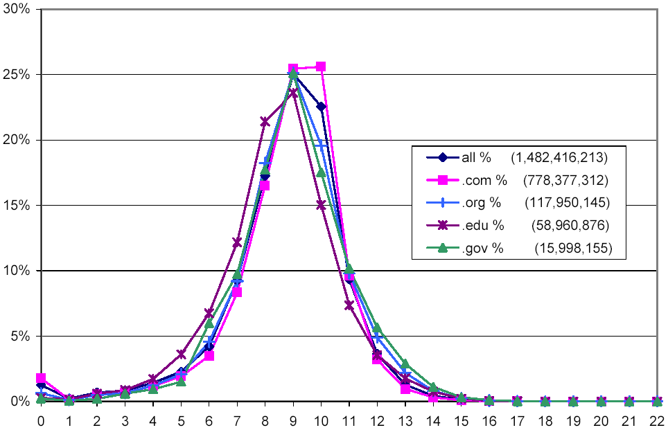
Figure 3: Distribution of words per documents overall and for selected top-level domains.
Figures 4, 5, and 6 attempt to capture different aspects of the permanence of web pages.
Figure 4 shows for each crawl generation the percentage of page retrievals resulting in different categories of status codes. The 200 category (corresponding to the HTTP status code "200 OK") shows pages that were successfully downloaded. Note that the y-axis starts at 85%; in all generations, over 85% of the retrievals were successful. The 3xx category contains all those pages that return an HTTP status code indicating that the page has moved. Since all URLs in our set produced a status code of 200 during crawl 1, the page has moved since. The 4xx category contains all client errors. The most common one is 404 ("Not Found"), indicating that the page has disappeared without leaving a forwarding address, distantly followed by 403 ("Forbidden"). The other category contains all pages for which the web server returned a status code not listed above. The various 5xx return codes dominated; we also found many web servers returning status codes not listed in the HTTP RFC. The network category contains all retrieval attempts that failed due to a network-related error, such as DNS lookup failure, refused connections, TCP timeouts, and the like (note that Mercator makes five attempts to resolve a domain name, and three attempts at retrievals that fail due to TCP errors). The RobotExcl category contains all those pages that were blocked by the web server's robots.txt file, and that we therefore refrained from even attempting to download. Again, since these pages were not excluded during crawl 1, the exclusion was imposed later. This appears to be a form of the Heisenberg effect, where the existence of an observer (a pesky web crawler that trots by every week) changes the behavior of the observed.
As one might expect, Figure 4 bears out that the lifetime of a URL is not unlimited. As the crawl generations increase, more and more URLs move, become unreachable, or are blocked from us. While one would expect a geometric progression of these trends, we did not observe the web long enough to distinguish the trend from a linear progression. The growth of these three categories comes at the expense of the 200 category; fluctuations in the share of the network category appear better correlated with network conditions at the crawler side.
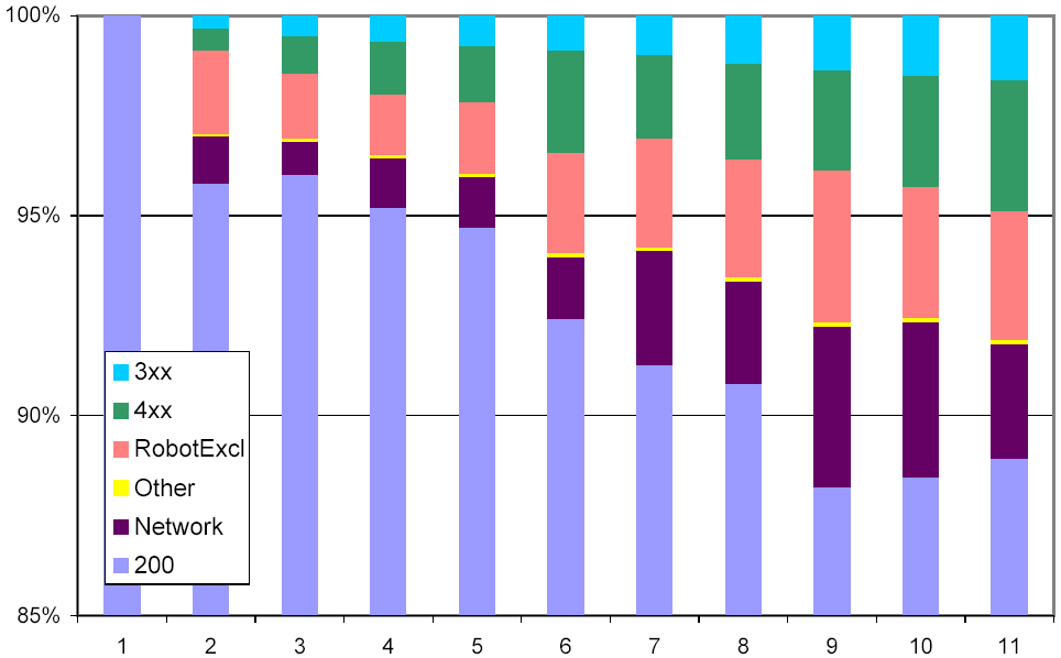
Figure 4: Distribution of HTTP status codes over crawl generations.
Figure 5 shows only the successful downloads as a percentage of all download attempts (including non-attempts due to robot exclusion rules), broken down by a few selected top-level domains. Note that the y-axis starts at 80%, reflecting the fact that all domains in all generations had at least that level of success. In general, pages in .jp, .de, and .edu were consistently more available than pages in .net and .com. The decline in the curves bears out the limited lifetime of web pages discussed above.
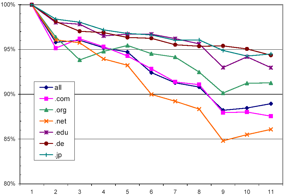
Figure 5: Distribution of successful downloads over crawl generations, broken down by selected top-level domains.
In Figure 6 we tried another approach for viewing the lifetime of URLs from different domains. Each bar represents a top-level domain (the leftmost bar represents the entire data set). We grouped URLs by the crawl generation of their last successful retrieval, the intuition being that a URL which could not be downloaded after some point is likely to have expired. This approach partitions URLs into 11 sets. Each shaded region of each bar represents the relative size of one such set. The region at the top of a bar corresponds to URLs that were consistently unreachable after crawl 1 (the crawl that defined the set of URLs), while the region at the bottom of a bar corresponds to URLs that were successfully downloaded during the final crawl. Note that the y-axis, which shows the percentage breakdown of the total, starts at 75%, due to the fact that for all domains considered here, more than 75% of all URLs were still reachable during the final crawl. Looking at the "all domains" bar, it can be seen that 88% of all URLs were still available during the final crawl.
For most domains, the "OK at crawl 10" regions are larger than regions for preceding crawls. This makes intuitive sense: it represents documents that could not be retrieved during the final crawl, but might well come back to life in the future. Other than that, we see no discernible patterns between the lengths of regions within a bar.
Looking across domains, we observe that web pages in China expire sooner than average, as do pages in .com and .net.
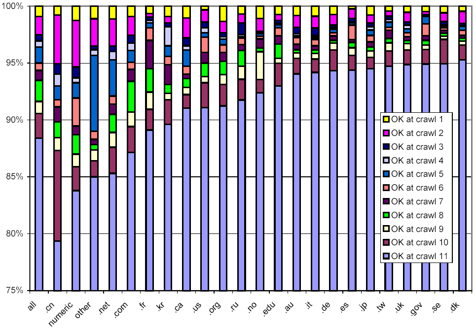
Figure 6: Breakdown showing in which crawl a web page was last successfully downloaded, broken down by TLD.
The remaining figures display information about the amount of change in a document between two successive successful downloads. Figure 7 shows a fine-grained illustration of change amount, independent of other factors. We partition the set of all pairs of successive successfully retrieved pages into 85 subsets, based on how many pre-images the two documents in each pair share. Subset 0 contains the pairs with no common pre-images, subset 84 the ones with all common pre-images, and subset 85 the ones that also agree in their document checksums (strongly suggesting that the documents are identical as byte sequences).
The x-axis shows the 85 subsets, and the y-axis shows percentages. The lower curve (visible only at the extreme left and right) depicts what percentage of all documents fall into a given subset. The curve above shows the cumulative percentage distribution. Each point (x,y) on the curve indicates that y percent of all pairs had at least x pre-images in common.
As can be seen (if your eyes are sharp enough), 65.2% of all page pairs don't differ at all. Another 9.2% differ only in their checksum, but have all common pre-images (suggesting that only the HTML markup, which was removed before computing pre-images, has changed).
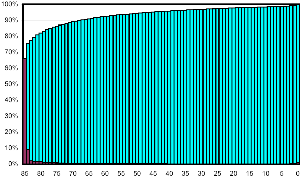
Figure 7: Distribution of change.
Figure 8 magnifies the lower curve from Figure 7, making it easy to see that all other change buckets contain less than 2% of all page pairs, and that all buckets with fewer than 79 common pre-images (representing document pairs that are less than 94% similar) contain less than 1%. For the most part, the curve is monotonically decreasing, but this pattern is broken as we get to the buckets containing documents that underwent extreme change. Bucket 0, which represents complete dissimilarity, accounts for 0.8%, over ten times the level of bucket 7, the smallest bucket. We will revisit this phenomenon later on.
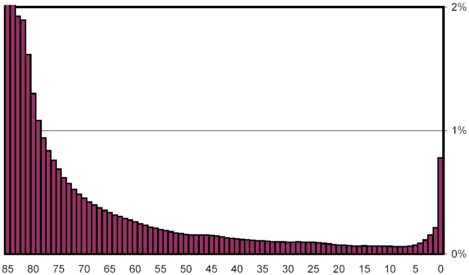
Figure 8: Distribution of change, scaled to show low-percentage categories.
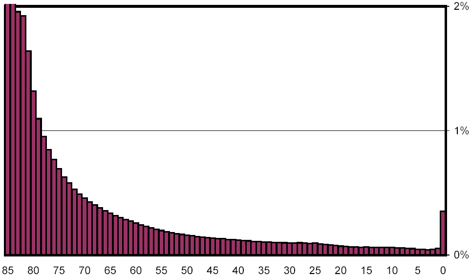
Figure 9: Distribution of change, scaled to show low-percentage categories, after excluding automatically generated keyword-spam documents.
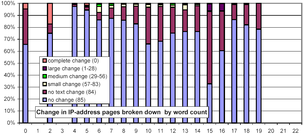
We next tried to determine if there are any attributes of a document that help to predict its rate and degree of change. In Figure 10, we examine the relation between top-level domain and change. The figure shows a bar for all page pairs and several more for selected domains. Each bar is divided into 6 regions, corresponding to the following six change clusters: complete change (0 common pre-images), large change (1-28 common pre-images), medium change (29-56 common pre-images), small change (57-83 common pre-images), no text change (84 common pre-images), and no change (subset 85: 84 common pre-images and a common checksum).
The top region depicts the complete change cluster, the one at the bottom the no change cluster. The y-axis shows the percentage.
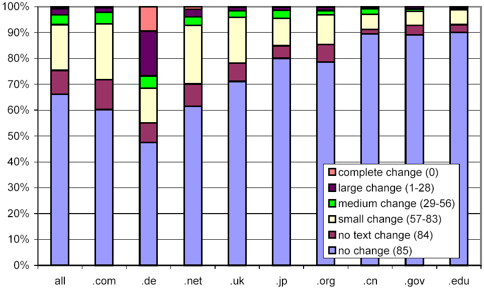
Figure 10: Clustered rates of change, broken down by selected top-level domains.
We observe significant differences between top-level domains, confirming earlier observations by Cho and Garcia-Molina [5]. In the .com domain, pages change more frequently than in the .gov and .edu domains.
We were surprised to see that pages in .de, the German domain, exhibit a significantly higher rate and degree of change than those in any other domain. 27% of the pages we sampled from .de underwent a large or complete change every week, compared with 3% for the web as a whole. Even taking the fabled German industriousness into account, these numbers were hard to explain.
In order to shed light on the issue, we turned to our sampled documents, selecting documents from Germany with high change rate. Careful examination of the first few pages revealed more than we cared to see: of the first half dozen pages we examined, all but one contained disjoint, but perfectly grammatical phrases of an adult nature together with a redirection to an adult web site. It soon became clear that the phrases were automatically generated on the fly, for the purpose of "stuffing" search engines such as Google with topical keywords surrounded by sensible-looking context, in order to draw visitors to the adult web site. Upon further investigation, we discovered that our data set contained 1.03 million URLs drawn from 116,654 hosts (4,745 of them being outside the .de domain), which all resolved to a single IP address. This machine is serving up over 15% of the .de URLs in our data set!
We speculate that the purpose of using that many distinct host names as a front to a single server is to circumvent the politeness policies that limit the number of pages a web crawler will attempt to download from any given host in a given time interval, and also to trick link-based ranking algorithms such as PageRank into believing that links to other pages on apparently different hosts are non-nepotistic, thereby inflating the ranking of the pages in the clique.
After this discovery, we set out to explore if there were other such servers in our data set. We resolved the symbolic host names of all the URLs in our data set, and singled out each IP address with more than a thousand symbolic host names mapping to it. There were 213 such IP addresses, 78 of which proved to be of a similar nature as the site that triggered our investigation. We excluded all URLs on the 443,038 hosts that resolved to one of the 78 identified IP addresses, and reran the analysis that produced Figure 10. This eliminated about 60% of the excessive large and complete change in .de. The adjusted distribution is shown in Figure 11. Continued investigation of the excessive change found that automatically generated pornographic content accounts for much of the remainder.
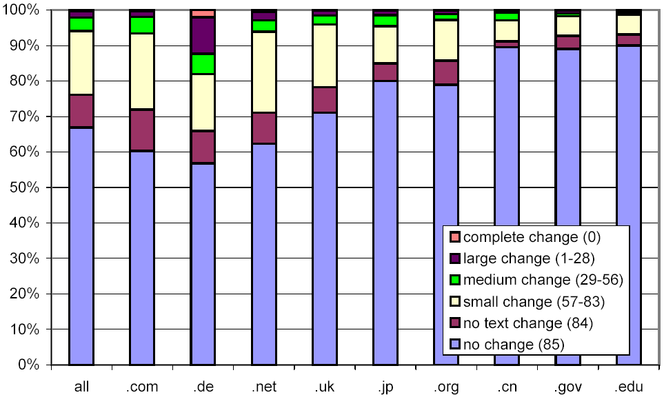
Figure 11: Clustered rates of change, broken down by selected top-level domains, after excluding automatically generated keyword-spam documents.
In Figure 12, we look at the same data, but omit all pairs of documents with no change. Other than Germany (and to a lesser extent China and Japan), there is remarkably little difference between the various top-level domains. Our conclusions are twofold: First, pornography continues to skew our results. Second, our shingling technique is not well adapted to writing systems like Chinese or Kanji that do not employ inter-word spacing, which in turn causes documents to have a very small number of shingles, which means that any change is considered significant.
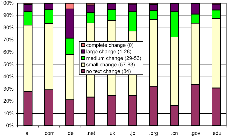
Figure 12: Clustered rates of change, broken down by selected top-level domains, and omitting the no change cluster.
Figure 9 is similar to Figure 8, but excludes the same URLs that were excluded in Figures 11 and 12. Note that most of the non-monotonicity at the right end of the distribution has disappeared, except for bucket 0, which nonetheless has been cut in half.
We next consider whether the length of pages impacts their rate of change. In Figure 13, we use the same x-axis semantics as in Figure 2, and the same y-axis semantics and bar graph encodings as in Figure 10. The most striking feature of this figure is that document size is strongly related to amount and rate of change, and counterintuitively so! One might think that small documents are more likely to change, and if they do, change more severely (since any change is a large change). However, we found that large documents (32 KB and above) change much more frequently than smaller ones (4 KB and below).
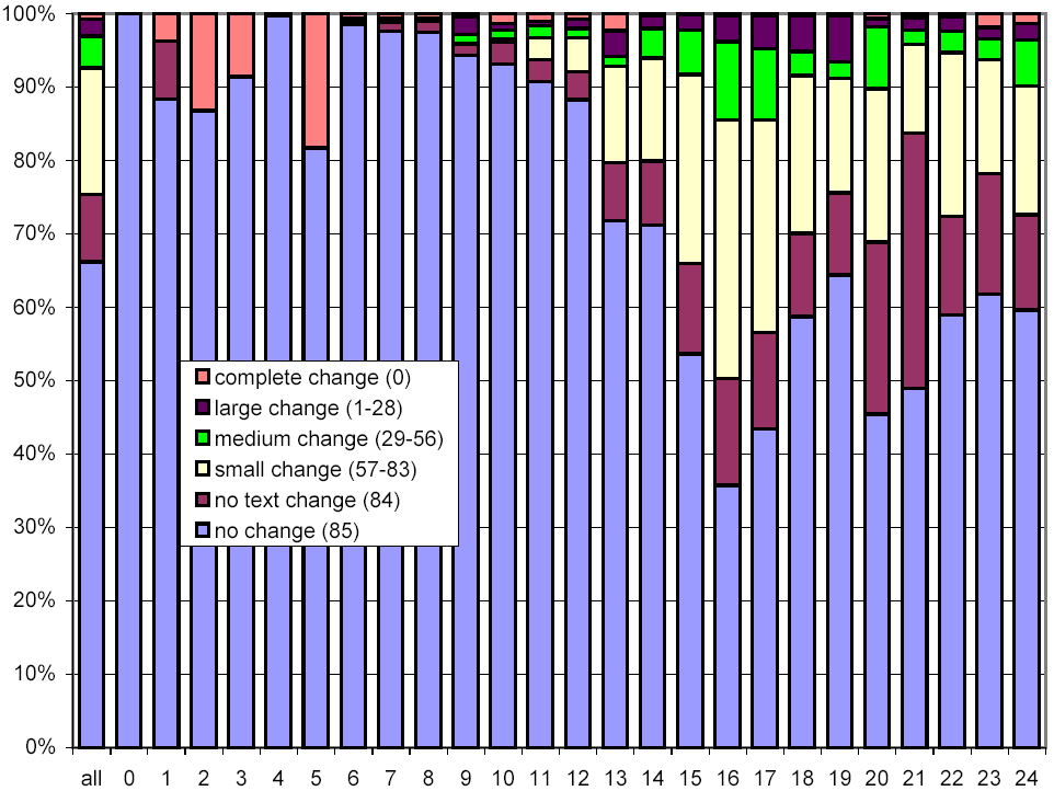
Figure 13: Clustered rates of change, broken down by document size.
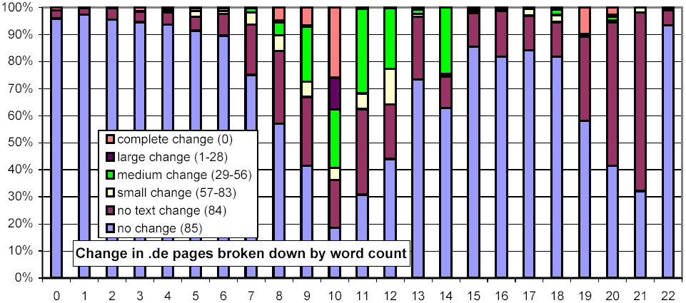
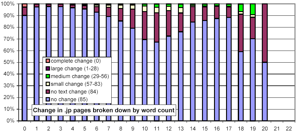
Figure 14 is similar in spirit, but examines the relationship between the number of words and the rate of change. In a way, this metric is more straightforward, since the sensitivity of our shingling techniques depends on the number of words in a document. For documents with few words, our metric gives a relatively coarse, "all-or-nothing" similarity metric. Nonetheless, this figure echoes the observation of Figure 13, that large documents are more likely to change than smaller ones.
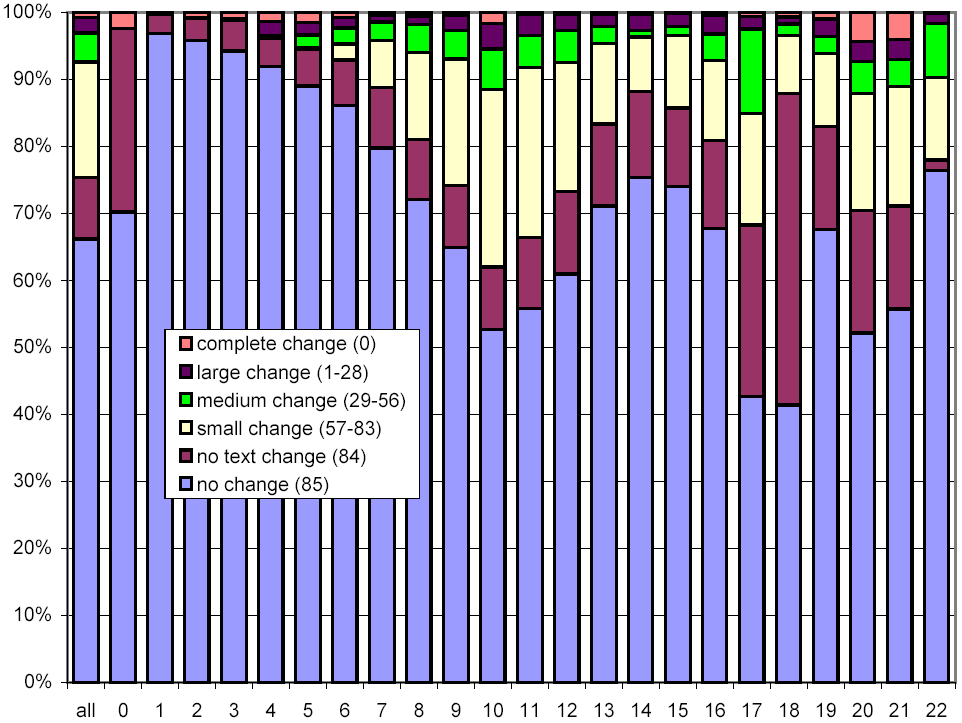
Figure 14: Clustered rates of change, broken down by number of words per document.
In Figure 15, we examine the same information, excluding the documents with no change. We observe that pages with different numbers of words exhibit similar change behavior, except that pages with just a few words cannot show an intermediate amount of change, due to our sampling technique.
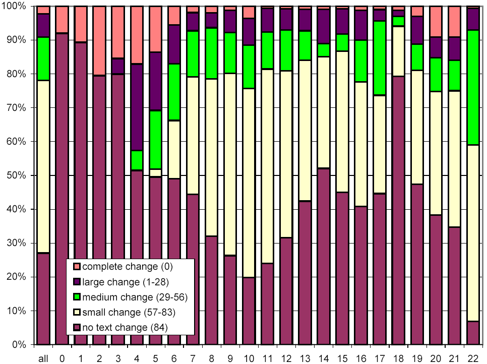
Figure 15: Clustered rates of change, broken down by number of words per document, and omitting the no change cluster.
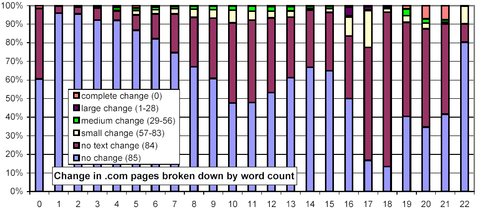
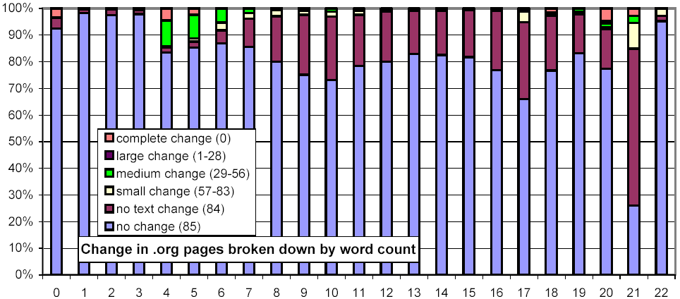
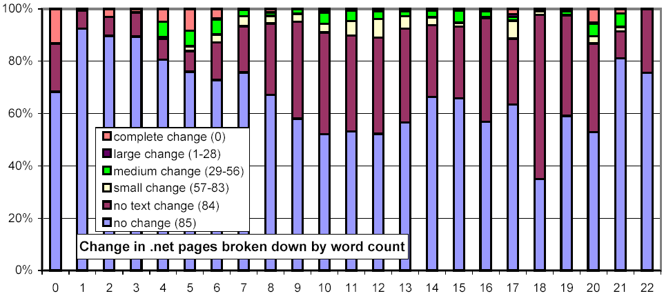
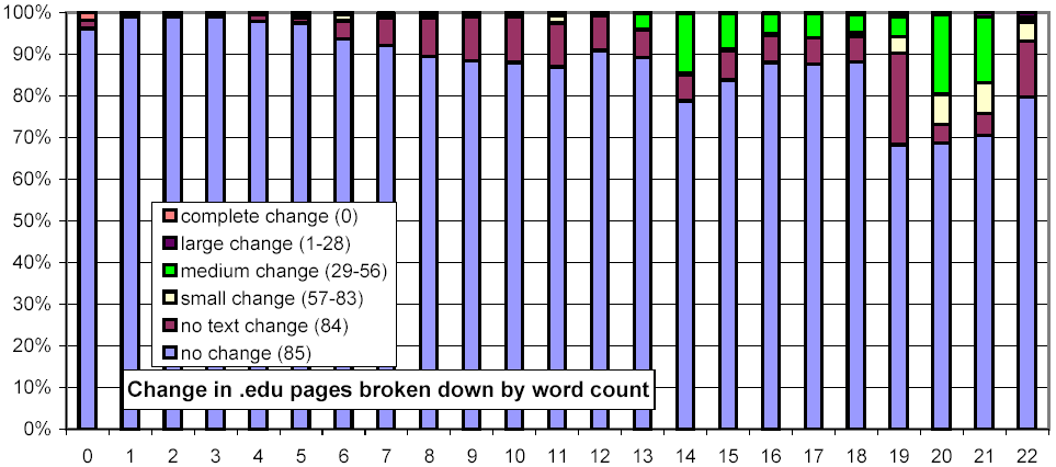
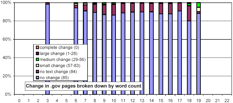
We further investigated whether there are any confounding relationships between document size and top-level domain. Figure 16 uses the same representation as Figure 13, but each chart considers only those URLs from a specific top-level domain. The distributions for the .com and .net domains exhibit a much stronger threshold effect for large documents than do .gov and .edu.
|
|
|
|
|
|
|
|
Figure 16: Clustered rates of change, broken down by top-level domain and number of words per document.
Figure 17 examines the correlation of successive changes to a document. The figure shows a 3D histogram. The x axis denotes the number of pre-images in a document unchanged from week n-1 to n, the y axis the number of pre-images unchanged from week n to n+1, and the z axis shows the logarithm (base 2) of the number of such documents. A data point (x,y,z) indicates that there are 2z document/week pairs (d,n) for which the versions of document d had x pre-images in common between weeks n-1 and n, and y pre-images in common between weeks n and n+1.
The spire surrounding the (x,y) coordinate (85,85) represents the vast majority of web pages that don't change much over a three-week interval. The tip of the spire is ten thousand times higher than any other feature in the plot, except for the smaller spire at the other end of the diagonal, which represents documents which differ completely in every sample. Much of this second peak can be attributed to machine-generated pornography, as described above.
The second-most prominent feature is the pronounced ridge along the main diagonal of the xy plane. The crest of the ridge represents a thousandfold higher number of instances per grid point than the floor of the valley. This ridge suggests that changes are highly correlated; past changes to a document are an excellent predictor of future changes.
The plumes at the far walls of the plot demonstrate that a sizable fraction of documents don't change in a given week, even if they changed in the previous or following week.
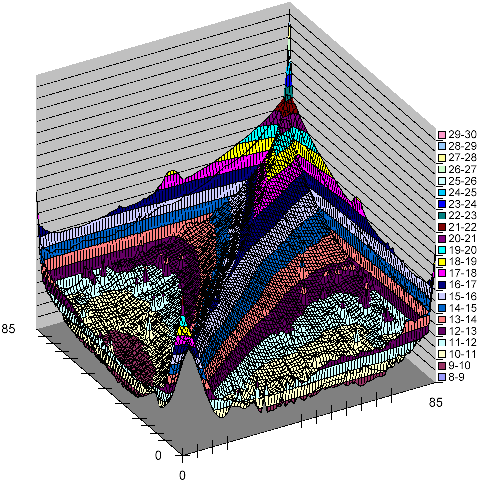
Figure 17: Logarithmic histogram of intra-document changes over three successive weeks, showing absolute number of changes.
Figure 18 modifies the previous figure in two ways: The view is down the z axis, transforming the 3D plot into a 2D contour map, where color/shading indicate the elevation of the terrain. In addition, rather than displaying absolute numbers of samples, we consider each column as a probability distribution (meaning that every data point is divided by the sum of the data points in its column). Since these values range from 0 to 1, their logarithms are negative. This normalization eliminates the spires that were so prominent in the previous figure. The diagonal ridge, however, remains, indicating once again that past change is a strong predictor of future change. Likewise, the plume along the top remains clearly visible.
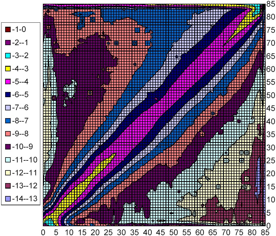
Figure 18: Logarithmic histogram of intra-document changes over three successive weeks, normalized to show conditional probabilities of changes.
This paper describes a large-scale experiment aimed at measuring the rate and degree of web page changes over a significant period of time. We crawled 151 million pages once a week for eleven weeks, saving salient information about each downloaded document, including a feature vector of the text without markup, plus the full text of 0.1% of all downloaded pages. Subsequently, we distilled the retained data to make it more amenable to statistical analysis, and we performed a number of data mining operations on the distilled data.
We found that web pages that change usually either change only in their markup or in trivial ways. Moreover, we found that there is a strong relationship between the top-level domain and the frequency of change of a document, whereas the relationship between top-level domain and degree of change is much weaker.
To our great surprise, we found that document size is another strong predictor of both frequency and degree of change. Moreover, one might expect that any change to a small document would be a significant one, by virtue of small documents having fewer words, so that any word change affects a significant fraction of the shingles. Contrary to that intuition, we found that large documents change more often and more extensively than smaller ones.
We investigated whether the two factors - top-level domain and document size - were confounding, and discovered that for the most part, the relationship of document size and rate and degree of change are more pronounced for the .com and .net domains than for, say, the .edu and .gov domains, suggesting that they are not confounded.
We also found that past changes to a page are a good predictor of future changes. This result has practical implications for incremental web crawlers that seek to maximize the freshness of a web page collection or index.
We have done some limited experiments with the sampled full text documents to investigate some of our more perplexing results. These experiments helped us in uncovering a source of pollution in our data set, namely machine-generated pages constructed for the purpose of spamming search engines. We hope that future work using the sampled full text documents will provide us with additional insights.
1 This definition of identity differs from the standard definition. For example, a document A is considered identical to AA, the concatenation of A to itself. Similarly, given two documents A and B, document AB is identical to document BA.
2 We drew the 84 functions from a smaller space, which does not seem to be a problem in practice. Also, because we fixed them at the time when we wrote the feature vector extraction module, an adversary who had the code of that module could produce documents that would fool our metric.
3 We actually did encounter several documents whose content type changed during the time we observed them.