|
Copyright is held by the author/owner(s).
WWW2002, May 7-11, 2002, Honolulu, Hawaii, USA.
ACM 1-58113-449-5/02/0005.
We present an algorithm for translating XSLT programs into SQL. Our context is that of virtual XML publishing, in which a single XML view is defined from a relational database, and subsequently queried with XSLT programs. Each XSLT program is translated into a single SQL query and run entirely in the database engine. Our translation works for a large fragment of XSLT, which we define, that includes descendant/ancestor axis, recursive templates, modes, parameters, and aggregates. We put considerable effort in generating correct and efficient SQL queries and describe several optimization techniques to achieve this efficiency. We have tested our system on all 22 SQL queries of the TPC-H database benchmark which we represented in XSLT and then translated back to SQL using our translator.
Categories & Subject Descriptors:
H.2.3 [Database Management]: Languages---Query languages, H.2.4 [Database Management]: Systems---Query processing
General Terms: Algorithms, Design, Languages
Keywords: XSLT, SQL, XML, query optimization, virtual view, translation
Copyright is held by the author/owner(s).
WWW2002, May 7-11, 2002, Honolulu, Hawaii, USA.
ACM 1-58113-449-5/02/0005.
XSLT is an increasingly popular language for processing XML data. Based on a recursive paradigm, it is relatively easy to use for programmers accustomed to a functional recursive style of programming. While originally designed to serve as a stylesheet, to map XML into HTML, it is increasingly used in other applications, such as querying and transforming XML data.
Today most of the XML data used in enterprise applications originates from relational databases, rather than being stored natively. There are strong reasons why this will not change in the near future. Relational database systems offer transactional guarantees, which make them irreplaceable in enterprise applications, and come equipped with high-performance query processors and optimizers. There exists considerable investment in today's relational database systems as well as the applications implemented on top of them. The language these systems understand is SQL.
Techniques for mapping relational data to XML are now well understood. Research systems in XML publishing [2,8,10,15] have shown how to specify a mapping from the relational model to XML and how to translate XML queries expressed in XML-QL [7] or XQuery [3] into SQL.
In this paper we present an algorithm for translating XSLT programs into efficient SQL queries. We identify a certain subset of XSLT for which the translation is possible and which is rich enough to express databases-like queries over XML data. This includes recursive templates, modes, parameters (with some restrictions), aggregates, conditionals, and a large fragment of XPath. One important contribution of this paper is to identify a new class of optimizations that need to be done either by the translator, or by the relational engine, in order to optimize the kind of SQL queries that result from such a translation.
We argue that the XSLT fragment described here is sufficient for expressing database-like queries in XSLT. As part of our experimental evaluation we have expressed all 22 SQL queries in the TPC-H benchmark [6] in this fragment, and translated them into SQL using our system. In all cases we could express these queries in our fragment, but in some cases the query we generated from the XSLT program turned out to be significantly more complex than the original TPC-H counterpart.
Translations from XML languages to SQL have been considered before, but only for XML query languages, like XML-QL and XQuery. The distinction is significant; since XSLT is not a query language, its translation to SQL is significantly more complex. The reason is the huge paradigm gap between XSLT's functional, recursive paradigm, and SQL's declarative paradigm. An easy translation is not possible, and, in fact, it is easy to construct programs in XSLT that have no SQL equivalent.
As an alternative to translation, it is always possible to interpret any XSLT program outside the relational engine, and use the RDBMS only as an object repository. For example, the XSLT interpreter could construct XML elements on demand, by issuing one SQL query for every XML element that it needs. We assume, that we can formulate a SQL query to retrieve an XML element with a given ID. Such an implementation would end up reading and materializing the entire XML document most of the time. Also, this approach would need to issue multiple SQL queries for a single XSLT program. This slows down the interpretation considerably because of the ODBC or JDBC connection overhead. In contrast, our approach generates a single SQL query for the entire XSLT program, thus pushing the entire computation inside the relational engine. This is the preferred solution, both because it makes a single connection to the database server and because it enables the relational engine to choose the best execution strategy for that particular program.
As an example, consider the XSLT program below:
<xsl:template match="*">
   <xsl:apply-template/>
</xsl:template>

<xsl:template match="person[name=='Smith']">
   <xsl:value-of select="phone/text()"/>
</xsl:template>
The program makes a recursive traversal of the XML tree, looking for a person called Smith and returning his phone. If we interpret this program outside the relational engine we need to issue a SQL query to retrieve the root element, then one SQL query for each child, until we find a person element, etc. This naive approach to XSLT interpretation ends up materializing the entire XML document.
Our approach is to convert the entire XSLT program into one SQL query. The query depends on the particular mapping from the relational data to XML; assuming such a mapping, the resulting SQL query is:
SELECT person.phoneThis can be up to order of magnitudes faster than the naive approach. In addition, if there exists an index on name in the database, then the relational engine can further improve performance.
FROM person
WHERE person.name = "Smith"
The organization of the paper is as follows. In Section 2 we provide some examples of XSLT to SQL translation to illustrate the main issues. Section 3 describes the architecture of our translator, and while Section 4 describes the various components in detail. We discuss the optimizations done to produce efficient SQL queries in Section 5. Section 6 presents the results of the experiments on TPC-H benchmark queries. Sections 7 and 8 discuss related work and conclusions.
We illustrate here some examples of XSLT to SQL translations, highlighting the main issues. As we go along, the fragment of XSLT translated by us will become clear. Throughout this section we illustrate our queries on the well-known beers/drinkers/bars database schema adapted from [17], shown in Figure 1. We will assume it is exported in XML as shown in Figure 2. Notice that there is some redundancy in the exported XML data, for example bars are accessible either directly from drinkers or under beers.
We assume the XML document to be unordered, and do not support any XSLT expressions that check order in the input. For example the beers under drinkers form an unordered collection. It is possible to extend our techniques to ordered XML views, but this is beyond our scope here. Furthermore, we will consider only element, attribute, and text nodes in the XML tree, and omit from our discussion other kinds of nodes such as comments or processing instructions.
XPath [5] is a component of XSLT, and the translation to SQL must handle it. For example the XPath /doc/drinkers/name/text() returns all drinkers. The equivalent SQL is:
For a less obvious example, consider the query in Figure 3 with two SQL queries Q2 and Q2'. Q2 is not a correct translation of P2, because it returns all beers, while P2 returns only beers liked by some drinker. Indeed P2 and Q2' have the same semantics. In particular Q2' preserves the multiplicities of the beers in the same way as P2.
Q2' is much more expensive than Q2, since it performs two joins, while Q2 is a simple projection. In some cases we can optimize Q2' and replace it with Q2, namely when the following conditions are satisfied: every beer is liked by at least one drinker, and the user specifies that the duplicates in the answer have to be removed. In this case P2 and Q2 have the same semantics, and our system can optimize the translation and construct Q2 instead of Q2'. This is one of the optimizations we consider in Section 5.
The XPath fragment supported by our system includes the entire language except constructs dealing with order and reference traversals. For example a navigation axis like ancestor-or-self is supported, while following-sibling is not.
A basic XSLT program is a collection of template rules. Each template rule specifies a matching pattern and a mode. Presence of modes allows different templates to be chosen when the computation arrives on the same node.
Figure 4 shows an XSLT program that returns for every drinker with age less than 25, pairs of (drinker name, all beers having price > 10 that she likes). The program has 3 modes. In the first mode (the default mode is 0) all drinkers with age less than 25 are selected. In the second mode (mode =1), for those drinkers all beers priced less than 10 are selected. In the third mode the result elements are created.
In general templates and modes are also used to modularize the program. The corresponding SQL query is also shown.
![\begin{figure}\begin{pseudocode} \lt xsl:template match=''drinkers[age \lt 25 ]'... ... beers.price \lt 10 AND beers.name = likes.beer \end{pseudocode}\end{figure}](p226-jain_img5.png)
|
Both XSLT and XPath can traverse the XML tree recursively. Consider the XPath expression //barname that retrieves all barnames. In absence of XML schema information it is impossible to express this query in SQL, because we need to navigate arbitrarily deep in the XML document. (Some SQL implementations support recursive queries and can express such XSLT programs; we do not generate recursive SQL queries in this work.) However, in the case of XML data generated from relational databases, the resulting XML document has a non-recursive schema, and we can unfold recursive programs into non-recursive ones. Using the schema in Fig. 2, the unfolded XPath expression is /drinkers/beers/barname
Recursion can also be expressed in XSLT through templates. Given a non-recursive XML schema, this recursion can also be eliminated, by introducing additional XSLT templates and modes. We describe the general technique in Section 4.1.
In XSLT one can bind some value to a parameter in one part of the tree, then use it in some other part. In SQL this becomes a join operation, correlating two tables. For example, consider the query in Figure 5, which finds all drinkers with the same astrosign as ``Brian''. A parameter is used to pass the value of ``Brian's'' astrosign, which is matched against every drinker's astrosign.
In this example, the value stored in variable and parameters was a single node. In general, they can store node-sets (specified using XPath, for instance), and also results of another template call (analogous to temporary tables in SQL). Our translation of XSLT to SQL supports all possible values taken on by variables.
Both XSLT and SQL support aggregates, but there is a a significant difference: in XSLT aggregate operator is applied to a subtree of in the input, while in SQL it is applied to a group using a Group By clause. Consider the query in Figure 6, which finds for every drinker the minimum price of all beers she likes. In XSLT we simply apply min to a subtree. In SQL we have to Group By drinkers.name.
For a glimpse at the difficulties involved in translating aggregates, consider the query in Figure 7, which, for every age, returns the cheapest price of all beers liked by people of that age. In XSLT we first find all ages, and then for each age apply min to a node-set, which in this case in not a sub-tree. The correct SQL translation for the XSLT program is shown next followed by an incorrect translation. The difference is subtle. In XSLT we collect all ages, with their multiplicities. That is, if three persons are 29 years old, then there will be three results with 29. The wrong SQL query contains a single such entry. The correct SQL query has an additional GroupBy attribute (name) ensuring that each age occurs the correct number of times in the output. See also our discussion in Section 6.
Apart from those already mentioned, our translation also supports if-[else], for-each, and case constructs. The for-each construct is equivalent to iteration using separate template rules. The case construct is equivalent to multiple if statements.
The translation from this XSLT fragment into SQL poses some major challenges. First, we need to map from a functional programming style to a declarative style. Templates correspond to functions, and their call graph needs to be converted into SQL statements. Second, we need to cope with general recursion, both at the XPath level and in XSLT templates. This is not possible in general, but it is always possible when the XML document is generated from a relational database, which is our case. Third, parameters add another source of complexities, and they typically need to be converted into joins between values from different parts of the XML tree. Finally, XSLT-style aggregation needs to be converted into SQL-style aggregation. This often involves introducing Group By clauses and, sometimes, complex conditions in the Having clause.
Figure 8 illustrates a more complex example with aggregation and parameters. The query finds for every drinker the cheapest beer she likes and its price. Notice the major stylistic difference between XSLT and SQL. In XSLT we compute the minimum price, bind it to a parameter, then search for the beer with that price and retrieve its name. In SQL we use the Having clause.
Orthogonal to the translation challenge per se, we have to address the quality of the generated SQL queries. Automatically generated SQL queries tend to be redundant and have unnecessary joins, typically self-joins [16]). An optimizer for eliminating redundant joins is difficult to implement since the general problem, called query minimization, is NP-complete [4]. Commercial databases systems do not do query minimization because it is expensive and because users do not write SQL queries that require minimization. In the case of automatically generated SQL queries however, it is all too easy to overshoot, and create too many joins. Part of the challenge in any such system is to avoid generating redundant joins.
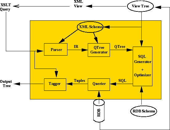
Figure 9 shows the architecture of the translator. An XML view is defined over the relational database using a View Tree [10]. The XML view typically consists of the entire database, but can also be a subset to export a subset view of the relational database. It can also include redundant information. The view never computed, but instead is kept virtual. Once the View Tree has been defined, the system accepts XSLT programs over the virtual XML view, and translates them to SQL in several steps.
First, the parser translates the XSLT program into an intermediate representation (IR). The IR is a DAG (directed acyclic graph) of templates with a unique root template (default mode template that matches `/'). Each leaf node contributes to the program's result, and each path from the root to a leaf node corresponds to a SQL query: the final SQL query is a union of all such queries. Each such path is translated first into a Query Tree (QTree) by the QTree generator. A QTree represents multiple, possible overlapping navigations through the XML document, together with selection, join, and aggregate conditions at various nodes. It is explained in Section 4.2.
The SQL generator plus optimizer takes a QTree as input, and generates an equivalent SQL query using the XML schema, RDB schema, and View Tree. The SQL generator is described in Section 4.4, and the optimizations are discussed in Section 5.
The querier has an easy task; it takes the generated SQL query and gets the resulting tuples from the RDB. The result tuples are passed onto the tagger, similar to [15], which produces the output for the user in a format dictated by the original query. The functionality of the querier and the tagger is straightforward and not our focus, and hence is not discussed further.
We will use as a running example the program in Figure 10, which retrieves the number of beers every drinker likes in common with Brian. We begin by describing how the XSLT program is parsed into an internal representation (IR) that reflects the semantics of the program in a functional style. We proceed to describe the QTree, which is an abstract representation of the paths traversed by the program on the View Tree. A QTree represents a single such path traversal, and is a useful intermediate representation for purposes of translating XML tree traversals into SQL. We describe our representation of the XML view over relational data (the View Tree, and finally show how we combine information from the QTree and View Tree to generate an equivalent SQL Query.
![\begin{figure}\begin{pseudocode} \lt xsl:template match=''drinkers''\gt \lt xsl... ...= $beerSet])/\gt \lt /result\gt \lt /\gt \lt /\gt \end{pseudocode}\end{figure}](p226-jain_img11.png)
|
The output of the parser is an Intermediate Representation (IR) of the XSLT query. Besides the strictly syntactic parsing, this module also performs a sequence of transformations to generate the IR. First it converts the XSLT program into a functional representation, in which each template mode is expressed as a function. Figure 11 (a) shows this for our running example. We add extra functions to represent the built-in XSLT template rules (Figure 11(b)), then we ``match'' the resulting program against the XML Schema (extracted from the View Tree). During the match all wildcards (*) are instantiated, all navigations other than parent/child are expanded into simple parent/child navigation steps, and only valid navigations are retained. This is shown in sequence in Figures 11 (c), (d) and (e). In some cases there may be multiple matches: Figure 12 (a) illustrates such an example, with the expansion in Figure 12 (b).
The end result for our running example is the IR shown in Figure 13. In this case the result is a single call graph. In some cases, a template calls more than one template conditionally (if-then-else or case constructs) or unconditionally (as shown in Figure 14). The semantics of such queries is the union of all possible paths that lead from the start template to a return node, as shown in Figure 14. .
At the end of the above procedure, we have one or more independent, straight-line call graphs. In what follows, we will demonstrate how to convert a straight-line call graph into a SQL query. The SQL query for the whole XSLT program is the union of the individual SQL queries.
The QTree is a simulation from the XML schema, and succinctly describes the computation being done by the query. The QTree abstraction captures the three components of an XML query: (a) the path taken by the query in the XML document, (b) the conditions placed on the nodes or data values along the path (c) the parameters passed between function calls. Corresponding to the three elements of the XML query above, a QTree has the following components.
Figure 15 (a) shows a QTree for the call graph in Figure 10. There are three QTrees in the figure. Q1 is the main QTree corresponding to the XSLT program. It has pointers to two other QTrees Q2 and Q3, which correspond to the two node-set parameters passed in the program.
The logic encapsulated by the XSLT program is as follows:
These steps correspond to the main QTree for the query Q1. Note that in step 3, when the query starts at the root to go to drinkers again, a separate drinker node is instantiated since the query could be referring to a drinker that is different from the current one (the root has multiple instances of ``drinker'' child nodes). QTrees are also created for every node-set. For example, the second parameter of the return call (count(beer[name == $...])) is represented as the QTree Q3. The predicate condition in the XPath for this parameter is represented in the QTree and refers to P1, defined in Q1.
As an abstraction, QTree is general enough that it can also be used for other XML query languages like XQuery and XML-QL. QTree is a powerful and succinct representation of the query computation independent of the language in which the query was expressed in. Moreover, the conversion from QTree to SQL is also independent of the query language.
The View Tree defines a mapping from the XML schema to the relational tables. Our choice of the View Tree representation has been borrowed from SilkRoute [10]. The View Tree defines a SQL query for each node in the XML schema. Figure 16 shows the View Tree for the beers/drinkers/bars schema. The right hand side of each rule should be interpreted as a SQL query. The rule heads (e.g., Drinkers) denote the table name, and the arguments denote the column name. Same argument in two tables represents a join on that value.
The query for an XML schema node depends on all its ancestors. For example, in Figure 16 the SQL for beername depends on drinkers and bars. Correspondingly, the SQL query for a child node is always a superset of the SQL query of its parent. Put another way, given the SQL query for a parent node, one can construct the query for its child node by adding appropriate FROM tables and WHERE constraints. As discussed later, such representation is crucial to avoid redundant joins, and hence generate efficient SQL queries.
This section explains how we generate SQL from a QTree using the View Tree. As explained before, a QTree represents a traversal of nodes in the original query and constraints placed by query on these nodes. The idea is to generate the SQL query clauses corresponding to those traversals and constraints. This is a three step process. First, nodes of the QTree are bound to instances of relational tables. Second, the appropriate WHERE constraints are generated using the binding in the first step. Intuitively, the first step generates the FROM part of the SQL query and join constraints due to tree traversal. The second step generates all explicitly specified constraints. Finally, the bindings for the return nodes are used to generate the SELECT part. We next describe each of these steps.
A binding associates a relational table, column pair to a QTree node. This (table,column) pair can be treated as its ``value''. The binding step updates the list of tables required in the FROM clause and implicit tree traversal constraints in WHERE clause.
We carry out this binding in a top down manner to avoid redundant joins. Before a node is bound, all its ancestors should be bound. To bind a node, we instantiate new versions of each table present in the View Tree SQL query for the child. Tables and constraints presented in the SQL of parent are not repeated again. The node can now be bound to an appropriate table name (using table renamings if required) and field using the SQL information from the View Tree.
The end result of binding a node n is bindings for all nodes that lie on the path from the root to n, a value association for n of the form tablename.fieldname, a list of tables to be included in the FROM clause, and the implicit constraints due to traversal.
Recall that all explicit conditions encountered during query traversal are stored in the QTree. In this step, these conditions are ANDed together along with the constraints generated in the binding step.
A condition is represented in the QTree as a boolean tree with
expressions at leaves. These expressions are converted to
constraints by recursively traversing the expression, and at each
step doing the following:
1. Constant expression are used verbatim.
2. Pointer to a QTree node is replaced by its binding.
3. Pointer to a QTree (i.e., the expression is a node set) is
replaced by a nested SQL query which is generated by calling the
conversion process recursively on the pointed QTree.
The values (columns of some table) bound to the return nodes form the SELECT part of the SQL query. If the return node is a pointer to a QTree, it is handled as mentioned above and the query generated is used as a subquery.
Figure 15 shows the mapping of three QTrees in our example to SQL after these steps. Figure 17 shows the SQL generated by our algorithm for Q1 after these steps.
We now briefly explain how our choice of a View Tree representation helps in eliminating join conditions. For any two paths in the QTree , nodes that lie on both paths must have the same value. One simple approach would be two bind the two paths independently and then for each common node add equality conditions to represent the fact that values from both paths are the same. For example, consider a very simple query that retrieves all all drinkers younger than 25. Figure 18 shows the QTree for this query.
If we take the approach of binding the nodes independently, and then adding the SQL constraints we will have the following SQL query:
SELECT drinkers3.name
FROM drinkers2, drinkers3
WHERE   drinkers2.age < 25 AND
           drinkers2.name = drinkers3.name
In our approach however we first iterate over the common node, which is the drinkers node, and then add the conditions. This leads to a better SQL query, shown below.
SELECT drinkers.name
FROM drinkers
WHERE drinkers.age < 25
This redundant join elimination becomes more important for complex queries, when there are many nodes that lie on multiple paths from the root to leaves.
Automated query generation is susceptible to generating inefficient queries with redundant joins and nested queries. Our optimizations unnest subqueries and eliminate joins that are not necessary. Most (but not all) of the optimizations described here are general-purpose SQL query rewritings that could be done by an optimizer. There are three reasons why we address them here. First, these optimizations are specific to the kind of SQL queries that result from our translations, and therefore may be missed by a general purpose optimizer. Second, our experience with one popular, commercial database system showed that, indeed, the optimizer did not perform any of them. Finally, some of the optimizations described here do not preserve semantics in general. The semantics are preserved only in the special context of the XSLT to SQL translation, and hence cannot be done by a general-purpose optimizer.
This optimization applies to predicate expressions of the form a in b, where b is a node-set (subquery). It can be applied only when the expression is present as a conjunction with other conditions. By default our SQL generation algorithm (Section 4.4) will generate a SQL query for the node-set b. This optimization would unnest such a subquery. Whether or not the query can be unnested depends on the properties of the node-set b. There are three possibilities:
This is the simplest case. One can safely unnest the query as it will not change the multiplicity of the whole query. Figure 19 illustrates this case. Note that astrosign in the XPath expression is a node-set.
To determine if the node-set is a singleton set, we use the following test. The View Tree has information regarding whether a node can have multiple values relative to its parent (by specifying a `*'). If no node in the QTree for the node-set has a `*' in the XML schema, then it must be a singleton set.
If the subquery has no duplicates, the query will evaluate to `true' at most once for all the values in the set b. Hence one can unnest the query without changing multiplicity. Figure 20 illustrates this case, for the example query used in the previous section.
To determine if the node-set has no duplicates, we use the following test. If the QTree for the nodeset has no node with a `*' except at the leaf node, then it is a distinct set. The intuition is that the siblings nodes (with the same parent) in the document are unique. So if there is a `*' at an edge other than the leaf edge, uniqueness of the leaves returned by the query is not guaranteed.
When a node-set can have duplicates for example, //beers, as discussed in Section 2.1, unnesting the query might change the semantics. This is because the multiplicity of the resultant query will change if the condition a in b evaluates to true more than once. We do not unnest such a query.
This optimization unnests a subquery that uses aggregation by using GROUP-BY at the outer level. The optimization is applied for expressions of the form op b, where b is a node-set, and op is an aggregate operator like sum, min, max, count, avg. The observation is that the nested query is evaluated once for every iteration of outer query. We get the same semantics if we unnest the query, and GROUP-BY on all iterations of outer query. To GROUP-BY on all iterations of outer query we add keys of all the tables in the from clause of outer query to the GROUP-BY clause. The aggregate condition is moved into the HAVING clause. In SQL, the GROUP-BY clause must have all the fields which are selected by the query. Hence all the fields in SELECT clause are also added to the GROUP-BY clause.
If the outer query already uses GROUP-BY then the above optimization can not be applied. This also implies that for a QTree this optimization can be used only once. In our implementation we take the simple choice of applying the optimization the very first time we can.
Figure 21 illustrates this case, for the example query used in the previous section.
In this optimization, we transform the QTree itself. Long paths with unreferenced intermediate nodes are shortened, as shown in Figure 22. This helps in eliminating some redundant joins. The optimization is done during the binding phase. Before binding a node, we checked to see if a short-cut path from root to that node exists. A short-cut path is possible if no intermediate node in the path is referred to by any other part of the QTree except the immediate child and parents of that node on that path. If a condition is referring to an intermediate node or if an intermediate node has more than one child, it is incorrect to create a short-cut path. Also the View Tree must specify that such a short-cut is possible, and what rules to use to bind the node if a short-cut is taken. Once the edge has been shortened and nodes bound, rest of the algorithm proceeds as before.
We observed that this optimization also helps in making the final SQL query less sensitive to input schema. For example, if our beers/drinkers/bars schema had ``beers'' as a top level node, instead of being as a child node of Drinkers, then the same query would had been obtained without the reduction optimization.
In this section we try to understand how well our algorithm translates XSLT queries to SQL queries. We implemented our algorithm in Java using the JavaCC parser [11]. Evaluation is done using the TPC-H benchmark [6] queries. We manually translated the benchmark SQL queries to XSLT, and then generated SQL queries from the XSLT queries using our algorithm. In the process we try to gauge the strengths and limitations of our algorithm, study the impact of optimizations described in Section 5, and observe the effects of semantic differences between XSLT and SQL.
The TPC-H benchmark is established by the Transaction Processing Council (TPC). It is an industry-standard Decision Support test designed to measure systems capability to examine large volumes of data and execute queries with a high degree of complexity. It consists of 22 business oriented ad-hoc queries. The queries heavily use aggregation and other sophisticated features of SQL. The TPC-H specification points out that these queries are more complex than typical queries.
Out of the 22 queries, 5 require creation of an intermediate table followed by aggregation on its fields. The equivalent XSLT translation would require writing two XSLT programs, the second one using the results of first. While this is possible in our framework as described in Section 4, our current implementation only supports parameters that are bound to fragments of the input tree, or to computed atomic values. It does not support parameters bound to a constructed tree. For such queries we translated the SQL query for the intermediate table, which in most cases was the major part of the overall query, to XSLT. Another modification we made was that aggregates on multiple fields like sum(a*b) were taken as aggregate on a single new field sum(c).
Overall, our algorithm generated efficient SQL queries in most cases, some of which were quite complex. A detailed table describing the result of translation for individual queries is presented in Appendix A. We present a summary of results here.
Many queries that were not translated as efficiently as their original SQL version required grouping by intermediate output. This is not an artifact of our translation algorithm, but due to a language-level mismatch between XSLT and SQL. An XSLT query with identical result cannot be written for these queries. With appropriate extensions to XSLT to support GROUP-BY, one can generate queries with identical results. It is no coincidence that this issue is mentioned in the future requirements draft for XSLT [12].
In this section, we describe the utility of each of the three optimizations, mentioned in Section 5, in obtaining efficient queries.
SilkRoute [10,8] is an XML publishing system that defines an XML view over a relational database, then accepts XML-QL [7] queries over the view and translates them into SQL. The XML view is defined by a View Tree, an abstraction that we borrowed for our translation. Both XML-QL and SQL are declarative languages, which makes the translation somewhat simpler than for XSLT. A translation from XQuery to SQL is described in [14] and uses a different approach based on an intermediate representation of SQL.
A generic technique for processing structurally recursive queries in bulk mode is described in [1]. Instead of using a generic technique, we leveraged the information present in the XML schema. This elimination is related to the query pruning described in [9]. SQL query block unnesting for an intermediate language has been discussed in [13] in the context of the Starburst system.
We have described an algorithm that translates XSLT into SQL. By necessity our system only applies to a fragment of XSLT for which the translation is possible. The full language can express programs which have no SQL equivalent: in such cases the program needs to be split into smaller pieces that can be translated into SQL.
Our translation is based on a representation of the XSLT program as a query tree, which encodes all possible navigations of the program through the XML tree. We described a number of optimization techniques that greatly improve the quality of the generated SQL queries. We also validated our system experimentally on the TPC-H benchmark.
We are thankful to Jayant Madhavan and Pradeep Shenoy for helpful discussions and feedback on the paper.
Dan Suciu was partially supported by the NSF CAREER Grant 0092955, a gift from Microsoft, and an Alfred P. Sloan Research Fellowship.
|